Ok

En poursuivant votre navigation sur ce site, vous acceptez l'utilisation de cookies. Ces derniers assurent le bon fonctionnement de nos services. En savoir plus.

10/03/2011

Algèbre sur un corps

Algèbre sur un corps

Source : http://fr.wikipedia.org/wiki/Alg%C3%A8bre_sur_un_corps

Cet article est une ébauche concernant les mathématiques.
Vous pouvez partager vos connaissances en l’améliorant (comment ?) selon les recommandations des projets correspondants.

Page d'aide sur l'homonymie Pour les articles homonymes, voir Algèbre (homonymie).

En mathématiques, une algèbre sur un corps commutatif K, ou simplement une K-algèbre, est une structure algébrique (A , + , . , × ) telle que :

  1. (A, +, ·) est un espace vectoriel sur K,
  2. la loi × est définie de A x A dans A (loi de composition interne)
  3. la loi × est distributive par rapport à la loi + .
  4. pour tout (ab) dans K2 et pour tout (xy) dans A2, (a·x)×(b·y) = (ab)·(x×y)

Définitions[modifier]

Soient K un corps commutatif et A un espace vectoriel sur K muni de plus d'une opération binaire (c'est-à-dire que le « produit » x×y de deux éléments de A est un élément de A. On dit que A est une algèbre sur K si cette opération binaire est distributive par rapport à + et bilinéaire, ce qui signifie que pour tous vecteurs x, y, z dans A et tous scalaires a, b dans K, les égalités suivantes sont vraies :

  • (x + y) z = x z + y z~,
  • x ( y + z) = x y + x z~,
  • (a x) (b y) = (a b) (x y)~.

On dit que K est le corps de base de A. L'opérateur binaire est souvent désigné comme la multiplication dans A.

Deux algèbres A et B sur K sont isomorphes s'il existe une bijection f:Ato B telle que

forall x,yin A,~forall ain K,~f(xy) = f(x) f(y)text{ et }f(x+ay) = f(x) + af(y)~.
Généralisation

Dans la définition, K peut être un anneau commutatif unitaire, et A un K-module. Alors, A est encore appelée une K-algèbre et on dit que K est l'anneau de base de A.

Article détaillé : algèbre sur un anneau.
Algèbres associatives, algèbres commutatives et alèbres unifères

Une algèbre associative est une algèbre sur un anneau dont la loi de composition interne x est associative. Lorsque cet anneau est un corps, il s'agit donc d'une

algèbre associative sur un corps (article détaillé).

Une algèbre est dite unifère si elle admet un élément neutre 1 pour la multiplication x. Une algèbre est dite commutative, si la loi de composition interne x est commutative.

Bases et tables de multiplication d'une algèbre sur un corps[modifier]

Tout espace vectoriel admet une base. Une base d'une algèbre A sur un corps K est une base de A pour sa structure d'espace vectoriel1.

Si a=(a_i)_{iin I} est une base de A, il existe alors une unique famille (c_{i,j}^k)_{i,j,k in I} d'éléments du corps K tels que :

displaystyle a_itimes a_j=sum_{kin I} c_{i,j}^k a_k.

Pour i et j fixés, les coefficients sont nuls sauf un nombre fini d'entre eux. On dit que (c_{i,j}^k)_{i,j,k in I} sont les constantes de structure1 de l'algèbre A par rapport à la base a, et que les relations a_itimes a_j=sum_{kin I} c_{i,j}^k a_k constituent la table de multiplication de l'algèbre A1.

Exemples d'algèbres de dimension finie[modifier]

Algèbres associatives et commutatives

Une base de l'algèbre mathbb C est constituée des éléments 1 et i. La table de multiplication est constituée des relations :

  • Tout corps fini est une algèbre associative, unifère et commutative de dimension n sur son sous-corps premier (mathbf F_p=mathbf Z / pmathbf Z), donc son ordre est pn.

Par exemple le corps fini mathbf F_4 est une algèbre de dimension 2 sur le corps mathbf F_2=mathbf Z / 2mathbf Z dont la table de multiplication dans une base (1, a) est :

  • On peut démontrer que toute algèbre unifère de dimension 2 sur un corps est associative et commutative2. Sa table de multiplication dans une base (1, x) est de la forme :

Une telle algèbre est appelée algèbre quadratique de type (a, b) (le type dépendant de la base choisie).

Algèbres associatives et non commutatives
  • L'ensemble des matrices carrées d'ordre ngeqslant2 à valeur dans mathbb Rleft(mathcal M_n(mathbb R), +,cdot, times right) est une mathbb R- algèbre associative, unifère et non commutative de dimension n2.
  • L'ensemble des quaternions (mathbb H, +,cdot, times) est une mathbb R- algèbre associative, unifère et non commutative de dimension 4.
  • L'ensemble des biquaternions (mathbb B, +,cdot, times) est une mathbb C-algèbre associative, unifère et non commutative de dimension 4 qui est isomorphe à l'algèbre left(mathcal M_2(mathbb C), +,cdot, times right) des matrices matrices carrées d'ordre 2 à valeur dans mathbb C.
Algèbre unifère non associative
  • L'ensemble des octonions (mathbb O, +,cdot, times) est une mathbb R- algèbre unifère non associative et non commutative de dimension 8.
Algèbres non associatives et non unifères
  • L'espace euclidien mathbb R^3 muni du produit vectoriel (mathbb R^3, +,cdot, wedge) est une mathbb R- algèbre non associative, non unifère et non commutative (elle est anti-commutative) de dimension 3.

La table de multiplication dans une base orthonormale directe (vec{u}vec{v}vec{w}) est :

  • L'ensemble des matrices carrées d'ordre ngeqslant2 à valeur dans mathbb R, muni du crochet de Lie : [M,N] = MN − NMleft(mathcal M_n(mathbb R), +,cdot, [,] right) est une mathbb R- algèbre non associative, nonunifère et non commutative de dimension n2. Elle est anti-commutative et possède des propriétés qui font de l'algèbre une algèbre de Lie.

Contre-exemple[modifier]

  • L'ensemble des quaternions (mathbb H, +,cdot, times) n'est pas une mathbb C-algèbre car la multiplication times n'est pas mathbb C-bilinéaire : icdot (jtimes k)neq jtimes (icdot k).

Voir aussi[modifier]

Notes et références[modifier]

  1. ↑ ab et c N. Bourbaki, Algèbre, chapitre III, p. 10.
  2.  N. Bourbaki, Algèbre, chapitre III, p. 13, proposition 1.

Sommaire

 [masquer]
1times 1=1, 1times i=i,
itimes 1=i, itimes i=-1
1times 1=1, 1times a=a,
atimes 1=a, atimes a=1+a
1times 1=1, 1times x=x,
xtimes 1=x, x2 = a1 + bx
vec{u}wedgevec{u} =vec{0}, vec{u}wedgevec{v} =vec{w}, vec{u}wedgevec{w} =-vec{v},
vec{v}wedgevec{u} =-vec{w}, vec{v}wedgevec{v} =vec{0}, vec{v}wedgevec{w} =vec{u},
vec{w}wedgevec{u} =vec{v}, vec{w}wedgevec{v} =-vec{u}, vec{w}wedgevec{w} =vec{0},

19:24 | Lien permanent | Commentaires (0) | |  del.icio.us | | Digg! Digg |  Facebook

Algèbre

Algèbre

Source : http://fr.wikipedia.org/wiki/Alg%C3%A8bre

Page d'aide sur l'homonymie Pour les articles homonymes, voir « Algèbre (homonymie) » et notamment la structure d'algèbre sur un anneau ou sur un corps.

L'algèbre, mot d'origine arabe al-jabr (الجبر), est la branche des mathématiques qui étudie les opérations et équations sur les nombres et plus généralement les structures algébriques.

L'étude de ces structures peut être faite de manière unifiée dans la cadre de l'algèbre universelle.

L'étude épistémologique de l'algèbre a été introduite par Jules Vuillemin.

Histoire[modifier]

Article détaillé : Chronologie de l'algèbre.

Antiquité[modifier]

Les anciens Babyloniens et Égyptiens savaient déjà résoudre des problèmes qui peuvent être traduits en équations du premier ou second degré.

Par exemple, le Papyrus Rhind (conservé au British Museum de Londres, il date de -1650, ère chrétienne) comporte l'énoncé suivant :

On doit diviser 100 miches de pain entre dix hommes comprenant un navigateur, un contremaître et un gardien, tous trois recevant double part. Que faut-il donner à chacun ?

Cependant, ils ne faisaient pas de l'algèbre, car ils n'effectuaient pas de calcul sur une inconnue.

Diophante d'Alexandrie (vers 200/214 - vers 284/298), au IIIe siècle de l'ère chrétienne, fut le premier à pratiquer l'algèbre en introduisant le concept d'inconnue en tant que nombre,1 et à ce titre peut être considéré comme "le père" de l'algèbre.

Monde arabo-musulman[modifier]

Page d'Algebra d'al-Khwarizmi

Le mot « algèbre » vient de l'arabe al-jabr (الجبر), qui est devenu algebra en latin et qui signifie « la réunion » (des morceaux), « la reconstruction » ou « la connexion » (en espagnol le mot algebrista désigne celui qui pratique le calcul algébrique mais aussi le rebouteux, celui qui sait réduire les fractures osseuses2).

C'est un des premiers mots du titre en arabe d'un ouvrage du mathématicien d'origine persane Al-Khawarizmi. Le titre de cet ouvrage (Al-jabr wa'l-muqabalah) qui s'inscrivait dans l'époque d'essor des sciences et techniques islamiques (la culture de l'époque voulait que tout savoir soit traduit en arabe et disséminé dans tout l'Empire), a donné le mot moderne « algèbre ». Une large proportion des méthodes utilisées sont issues de résultats élémentaires de géométrie. Pour cette raison, on classe souvent ces premiers résultats dans la branche de l'algèbre géométrique.

Après un voyage dans le nord de l'Afrique, Léonard de Pise dit Fibonacci fut séduit par cette nouvelle façon d'écrire les chiffres (différente des chiffres romains) et par le système décimal. Dès son retour au pays, il est parmi les premiers à populariser les chiffres arabes et le système décimal en Europe et travaille sur sa fameuse suite.

XVIe siècle : Europe[modifier]

Le pape Gerbert d'Aurillac avait ramené d'Espagne vers l'an 1000 le zéro, invention indienne que les mathématiciens Al-Khawarizmi et Abu Kamil avaient eux-mêmes fait connaître dans tout l'Empire, et aussi à Cordoue.

Cette numération de position lance une ère de calcul algébrique, d'abord au moyen des algorithmes nommés ainsi en hommage à Al-Kawarizmi, qui remplacent peu à peu l'usage de l'abaque. Les mathématiciens italiens du XVIe siècle (del FerroTartaglia et Cardan) résolvent l'équation du 3e degré (ou équation cubique).Ferrari, élève de Cardan, résout l'équation du 4e degré (ou équation quartique), et la méthode est perfectionnée par Bombelli. À la fin du siècle, le Français Viètedécouvre que les fonctions symétriques des racines sont liées aux coefficients de l'équation polynomiale.

Jusqu'au xviie siècle, l'algèbre peut être globalement caractérisée comme la suite ou le début des équations et comme une extension de l'arithmétique ; elle consiste principalement en l'étude de la résolution des équations algébriques, et la codification progressive des opérations symboliques permettant cette résolution. C'est à François Viète (1540-1603) que l'on doit l'idée de noter les inconnues numériques à l'aide de lettres .

Au XVIIe siècle, les mathématiciens utilisent progressivement des nombres « imaginaires », tels que l'une des racines carrées de -1, pour parvenir à calculer les racines non réelles de leurs équations. Cette « extension » des nombres réels (qui prendra le nom de nombres complexes) amène d'Alembert (en 1746) etGauss (en 1799) à énoncer et démontrer le théorème fondamental de l'algèbre (ou théorème de d'Alembert-Gauss) :

Théorème — Toute équation polynomiale de degré n en nombres complexes a exactement n racines (en comptant chacune avec son éventuelle multiplicité).

Sous sa forme moderne, le théorème s'énonce :

Théorème — Le corps  _mathbb C  des nombres complexes muni de l'addition et de la multiplication est algébriquement clos.

Le XIXe siècle s'intéresse désormais à la calculabilité des racines, et en particulier à la possibilité de les exprimer par des formules générales à base de radicaux. Les échecs concernant les équations de degré 5 amènent le mathématicien Abel (après VandermondeLagrange et Gauss) à approfondir les transformations sur l'ensemble des racines d'une équation. Évariste Galois (1811 - 1832), dans un mémoire fulgurant, introduit pour la première fois la notion de groupe (en étudiant le groupe des permutations des racines d'une équation polynomiale) et aboutit à l'impossibilité de la résolution par radicaux pour les équations de degré supérieur ou égal à 5.

Une étape décisive était franchie avec l'écriture des exposants fractionnaires. Celle-ci permettra à Euler d'énoncer sa célèbre formule eiπ + 1 = 0 liant cinq nombres remarquables.

Algèbre moderne[modifier]

Dès lors, l'algèbre moderne entame un parcours fécond : Boole crée l'algèbre qui porte son nomHamilton invente les quaternions, et les mathématiciens anglais CayleyHamilton et Sylvester étudient les structures de matrices. L'algèbre linéaire, longtemps restreinte à la résolution de systèmes d'équations linéaires à 2 ou 3 inconnues, prend son essor avec le théorème de Cayley-Hamilton (« Toute matrice carrée à coefficients dans  _mathbb R  ou  _mathbb C  annule son polynôme caractéristique »). S'ensuivent les transformations par changement de base, la diagonalisation et la trigonalisation des matrices, et les méthodes de calcul qui nourriront, au XXe siècle, la programmation des ordinateurs. Parallèlement, Kummer généralise les structures galoisiennes et étudie les structures de corps et d'anneau. Dedekind définit les idéaux (déjà entrevus par Gauss) qui permettront de généraliser et reformuler les grands théorèmes d'arithmétique. L'algèbre linéaire se généralise en algèbre multilinéaire et algèbre tensorielle.

Au début du XXe siècle, sous l'impulsion de l'allemand Hilbert et du français Poincaré, les mathématiciens s'interrogent sur les fondements des mathématiques :logique et axiomatisation occupent le devant de la scène. Peano axiomatise l'arithmétique, puis les espaces vectoriels. La structure d'espace vectoriel et lastructure d'algèbre sont approfondies par Artin en 1925, avec des corps de base autres que  _mathbb R  ou  _mathbb C  et des opérateurs toujours plus abstraits. On doit aussi àArtin, considéré comme le père de l'algèbre contemporaine, des résultats fondamentaux sur les corps de nombres algébriques. Les corps non commutatifs amènent à définir la structure de module sur un anneau et la généralisation des résultats classiques sur les espaces vectoriels.

L'école française « Nicolas Bourbaki », emmenée par WeilCartan et Dieudonné, entreprend de réécrire l'ensemble des connaissances mathématiques sur une base axiomatique : ce travail gigantesque commence par la théorie des ensembles et l'algèbre dans le milieu du siècle, et confirme l'algèbre comme langage universel des mathématiques. Paradoxalement, alors que le nombre de publications suit une croissance exponentielle à travers le monde, alors qu'aucun mathématicien ne peut prétendre dominer qu'une toute petite partie des connaissances, les mathématiques n'ont jamais autant paru unifiées qu'aujourd'hui.

Notations européennes modernes[modifier]

Voir aussi[modifier]

Sur les autres projets Wikimédia :

Notes et références[modifier]

  1.  Diophante et l'algèbre pré-symbolique [archive], Luis RADFORD .
  2.  Diccionario de la lengua española [archive] de la Real Academia Española

Bibliographie[modifier]

  • Adolf P. Youschkevitch, Les Mathématiques Arabes, VIIIe-XVe siècles, Ed. VRIN, Paris - 1976

Liens externes[modifier]

Sommaire

 [masquer]

19:23 Publié dans Algèbre | Lien permanent | Commentaires (0) | |  del.icio.us | | Digg! Digg |  Facebook

08/03/2011

Pythagorean theorem

Pythagorean theorem

From Wikipedia, the free encyclopedia Source : 
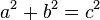
The Pythagorean theorem: The sum of the areas of the two squares on the legs (aand b) equals the area of the square on the hypotenuse (c).

In mathematics, the Pythagorean theorem or Pythagoras' theorem is a relation in Euclidean geometry among the three sides of a right triangle (right-angled triangle). In terms of areas, it states:

In any right triangle, the area of the square whose side is the hypotenuse (the side opposite the right angle) is equal to the sum of the areas of the squares whose sides are the two legs (the two sides that meet at a right angle).

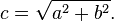
The theorem can be written as an equation relating the lengths of the sides ab and c, often called the Pythagorean equation:[1]

a^2 + b^2 = c^2!,

where c represents the length of the hypotenuse, and a and b represent the lengths of the other two sides.

These two formulations show two fundamental aspects of this theorem: it is both a statement about areas and about lengthsTobias Dantzigrefers to these as areal and metric interpretations.[2][3] Some proofs of the theorem are based on one interpretation, some upon the other. Thus, Pythagoras' theorem stands with one foot in geometry and the other in algebra, a connection made clear originally by Descartes in his work La Géométrie, and extending today into other branches of mathematics.[4]

The Pythagorean theorem has been modified to apply outside its original domain. A number of these generalizations are described below, including extension to many-dimensional Euclidean spaces, to spaces that are not Euclidean, to objects that are not right triangles, and indeed, to objects that are not triangles at all, but n-dimensional solids.

The Pythagorean theorem is named after the Greek mathematician Pythagoras, who by tradition is credited with its discovery and proof,[5][6] although it is often argued that knowledge of the theorem predates him. (There is much evidence that Babylonian mathematicians understood the formula, although there is little surviving evidence that they fitted it into a mathematical framework.[7]) "[To the Egyptians and Babylonians] mathematics provided practical tools in the form of 'recipes' designed for specific calculations. Pythagoras, on the other hand, was one of the first to grasp numbers as abstract entities that exist in their own right."[8]

The Pythagorean theorem has attracted interest outside mathematics as a symbol of mathematical abstruseness, mystique, or intellectual power. Popular references to Pythagoras' theorem in literature, plays, musicals, songs, stamps and cartoons abound.

[edit]Other forms

As pointed out in the introduction, if c denotes the length of the hypotenuse and a and b denote the lengths of the other two sides, Pythagoras' theorem can be expressed as the Pythagorean equation:

a^2 + b^2 = c^2,

or, solved for c:

 c = sqrt{a^2 + b^2}. ,

If c is known, and the length of one of the legs must be found, the following equations can be used:

b = sqrt{c^2 - a^2}. ,

or

a = sqrt{c^2 - b^2}. ,

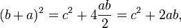
The Pythagorean equation provides a simple relation among the three sides of a right triangle so that if the lengths of any two sides are known, the length of the third side can be found. A generalization of this theorem is the law of cosines, which allows the computation of the length of the third side of any triangle, given the lengths of two sides and the size of the angle between them. If the angle between the sides is a right angle, the law of cosines reduces to the Pythagorean equation.

[edit]Proofs

This theorem may have more known proofs than any other (the law of quadratic reciprocity being another contender for that distinction); the book The Pythagorean Proposition contains 370 proofs.[9]

[edit]Proof using similar triangles

Proof using similar triangles

This proof is based on the proportionality of the sides of two similar triangles, that is, upon the fact that the ratio of any two corresponding sides of similar triangles is the same regardless of the size of the triangles.

Let ABC represent a right triangle, with the right angle located at C, as shown on the figure. We draw the altitude from point C, and call H its intersection with the side AB. Point H divides the length of the hypotenuse c into parts d and e. The new triangle ACH is similar to triangleABC, because they both have a right angle (by definition of the altitude), and they share the angle at A, meaning that the third angle will be the same in both triangles as well, marked as θ in the figure. By a similar reasoning, the triangle CBH is also similar to ABC. The proof of similarity of the triangles requires the Triangle postulate: the sum of the angles in a triangle is two right angles, and is equivalent to the parallel postulate. Similarity of the triangles leads to the equality of ratios of corresponding sides:

 frac{a}{c}=frac{e}{a} mbox{ and } frac{b}{c}=frac{d}{b}.,

The first result equates the cosine of each angle θ and the second result equates the sines.

These ratios can be written as:

a^2=ctimes e mbox{ and }b^2=ctimes d. ,

Summing these two equalities, we obtain

a^2+b^2=ctimes e+ctimes d=ctimes(d+e)=c^2 ,,!

which, tidying up, is the Pythagorean theorem:

a^2+b^2=c^2  .,!

This is a metric proof in the sense of Dantzig, one that depends on lengths, not areas. The role of this proof in history is the subject of much speculation. The underlying question is why Euclid did not use this proof, but invented another. One conjecture is that the proof by similar triangles involved a theory of proportions, a topic not discussed until later in the Elements, and that the theory of proportions needed further development at that time.[10][11]

[edit]Euclid's proof

Proof in Euclid's Elements

In outline, here is how the proof in Euclid's Elements proceeds. The large square is divided into a left and right rectangle. A triangle is constructed that has half the area of the left rectangle. Then another triangle is constructed that has half the area of the square on the left-most side. These two triangles are shown to be congruent, proving this square has the same area as the left rectangle. This argument is followed by a similar version for the right rectangle and the remaining square. Putting the two rectangles together to reform the square on the hypotenuse, its area is the same as the sum of the area of the other two squares. The details are next.

Let ABC be the vertices of a right triangle, with a right angle at A. Drop a perpendicular from A to the side opposite the hypotenuse in the square on the hypotenuse. That line divides the square on the hypotenuse into two rectangles, each having the same area as one of the two squares on the legs.

For the formal proof, we require four elementary lemmata:

  1. If two triangles have two sides of the one equal to two sides of the other, each to each, and the angles included by those sides equal, then the triangles are congruent (side-angle-side).
  2. The area of a triangle is half the area of any parallelogram on the same base and having the same altitude.
  3. The area of a rectangle is equal to the product of two adjacent sides.
  4. The area of a square is equal to the product of two of its sides (follows from 3).

Next, each top square is related to a triangle congruent with another triangle related in turn to one of two rectangles making up the lower square.[12]

Illustration including the new lines

The proof is as follows:

  1. Let ACB be a right-angled triangle with right angle CAB.
  2. On each of the sides BC, AB, and CA, squares are drawn, CBDE, BAGF, and ACIH, in that order. The construction of squares requires the immediately preceding theorems in Euclid, and depends upon the parallel postulate.[13]
  3. From A, draw a line parallel to BD and CE. It will perpendicularly intersect BC and DE at K and L, respectively.
  4. Join CF and AD, to form the triangles BCF and BDA.
  5. Angles CAB and BAG are both right angles; therefore C, A, and G are collinear. Similarly for B, A, and H.
    Showing the two congruent triangles of half the area of rectangle BDLK and square BAGF
  6. Angles CBD and FBA are both right angles; therefore angle ABD equals angle FBC, since both are the sum of a right angle and angle ABC.
  7. Since AB and BD are equal to FB and BC, respectively, triangle ABD must be congruent to triangle FBC.
  8. Since A is collinear with K and L, rectangle BDLK must be twice in area to triangle ABD, since it shares a height with BK and a base with BD and a triangle's area is half the product of its base and height.
  9. Since C is collinear with A and G, square BAGF must be twice in area to triangle FBC.
  10. Therefore rectangle BDLK must have the same area as square BAGF = AB2.
  11. Similarly, it can be shown that rectangle CKLE must have the same area as square ACIH = AC2.
  12. Adding these two results, AB2 + AC2 = BD × BK + KL × KC
  13. Since BD = KL, BD* BK + KL × KC = BD(BK + KC) = BD × BC
  14. Therefore AB2 + AC2 = BC2, since CBDE is a square.

This proof, which appears in Euclid's Elements as that of Proposition 47 in Book 1,[14] demonstrates that the area of the square on the hypotenuse is the sum of the areas of the other two squares.[15] It is therefore an areal proof in the sense of Dantzig, one that depends on areas, not lengths. This makes it quite distinct from the proof by similarity of triangles, which is conjectured to be the proof that Pythagoras used.[11][16]

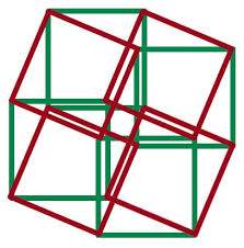
[edit]Proof by rearrangement

In the animation at the left, the total area and the areas of the triangles are all constant. Therefore, the total black area is constant. But the original black area of side c can be divided into two squares with sides ab, demonstrating that a2 + b2 = c2.

A second proof is given by the middle animation. An initial large square is formed of area c2 by adjoining four identical right triangles, leaving a small square in the center of the big square to accommodate the difference in lengths of the sides of the triangles. Two rectangles are formed of sides a and b by moving the triangles. By incorporating the center small square with one of these rectangles, the two rectangles are made into two squares of areas a2 and b2, showing that c2 = a2 + b2.

The third, rightmost image also gives a proof. The upper two squares are divided as shown by the blue and green shading, into pieces that when rearranged can be made to fit in the lower square on the hypotenuse – or conversely the large square can be divided as shown into pieces that fill the other two. This shows the area of the large square equals that of the two smaller ones.[17]

[edit]Algebraic proofs

Diagram of the two algebraic proofs.

The theorem can be proved algebraically using four copies of a right triangle with sides ab and c, arranged inside a square with side c as in the top half of the diagram.[19] The triangles are similar with area tfrac12ab, while the small square has side b − a and area (b − a)2. The area of the large square is therefore

(b-a)^2+4frac{ab}{2} = (b-a)^2+2ab = a^2+b^2. ,

But this is a square with side c and area c2, so

c^2 = a^2 + b^2. ,

A similar proof uses four copies of the same triangle arranged symmetrically around a square with side c, as shown in the lower part of the diagram.[20] This results in a larger square, with side a + b and area (a + b)2. The four triangles and the square side c must have the same area as the larger square,

(b+a)^2 = c^2 + 4frac{ab}{2} = c^2+2ab,,

giving

c^2 = (b+a)^2 - 2ab = a^2 + b^2.,
Diagram of Garfield's proof.

A related proof was published by James A. Garfield.[21][22] Instead of a square it uses a trapezoid, which can be constructed from the square in the second of the above proofs by bisecting along a diagonal of the inner square, to give the trapezoid as shown in the diagram. The area of the trapezoid can be calculated to be half the area of the square, that is

frac{1}{2}(b+a)^2.

The inner square is similarly halved, and there are only two triangles so the proof proceeds as above except for a factor of frac{1}{2}, which is removed by multiplying by two to give the result.

[edit]Proof using differentials

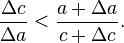
One can arrive at the Pythagorean theorem by studying how changes in a side produce a change in the hypotenuse and employing calculus.[23][24] This proof is a metric proof in the sense of Dantzig, as it uses lengths, not areas.

In the figure, triangle PBC is the original right triangle and triangle ABC is the modification of PBC when side PB is extended by increasing a to a + Δa. The circular arcs have radii c and c + Δc where Δc is the change in hypotenuse c that occurs as a result of the change Δa in side a.

Constructions to determine upper and lower bounds upon Delta c / Delta a , .[23]

The figure shows two constructions, right triangles ADP and AQP, in the upper and lower panels which will be used to find respectively upper and lower boundsof the ratio Δca. Then the limit will be taken as Δa, Δc → 0, and the resulting expression for the derivative dc /da will be used to establish Pythagoras' theorem.

From triangle ABC (upper panel),

cos theta = frac{AB}{AC} =  frac{a + Delta a}{c+Delta c}.

Construct right triangle ADP (upper panel). Then,

cos theta = frac{AD}{AP} = frac{AD}{Delta a} > frac{Delta c}{Delta a}.

The last inequality results from AD > Δc , as shown in the upper panel of the figure.[25] Combining the above expressions for cos θ,

frac{Delta c}{Delta a} < frac{a + Delta a}{c+Delta c}.

Next construct right triangle AQP (lower panel). Since both triangles AQP and PBC have an angle  scriptstyle phi ,

 cos phi = frac{a}{c} =frac{PQ}{PA}= frac{PQ}{Delta a}  < frac{Delta c}{Delta a}.

The last inequality results from PQ < Δc, as shown in the lower panel of the figure. Combining the two inequalities that were obtained using triangles ADP and AQP,

frac{a}{c} < frac{Delta c}{Delta a} < frac{a + Delta a}{c+Delta c} = left(frac{a}{c} right) frac{1+ Delta a /a}{1+Delta c /c}.

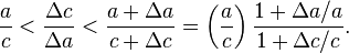
We now have upper and lower bounds for the ratio Δc /ΔaAs Δa, Δc → 0, the ratio Δc /Δa becomes the derivative dc /da and the upper bound becomes the same as the lower bounda /c. Consequently,

frac {dc}{da} =frac{a}{c},

or:

c , dc = a , da;   d (c^2) = d (a^2),

which has the integral:

 c^2 = a^2 + text{ constant}.,

When a = 0 then c = b, so the "constant" is b2. Hence, Pythagoras' theorem is established:

c^2 = a^2 + b^2.,

Using this expression, the total differential is:

 d(c^2) = d(a^2) +d(b^2).,

This result shows that the increase in the square of the hypotenuse is the sum of the independent contributions from the squares of the sides.

[edit]Converse

The converse of the theorem is also true:[26]

For any three positive numbers ab, and c such that a2 + b2 = c2, there exists a triangle with sides ab and c, and every such triangle has a right angle between the sides of lengths a and b.

Such numbers are called a Pythagorean triple. An alternative statement is:

For any triangle with sides abc, if a2 + b2 = c2, then the angle between a and b measures 90°.

This converse also appears in Euclid's Elements (Book I, Proposition 48):[27]

"If in a triangle the square on one of the sides equals the sum of the squares on the remaining two sides of the triangle, then the angle contained by the remaining two sides of the triangle is right."

It can be proven using the law of cosines (see below under Generalizations), or by the following proof:

Let ABC be a triangle with side lengths ab, and c, with a2 + b2 = c2. We need to prove that the angle between the a and b sides is a right angle. We construct a second triangle with sides of lengths a and b containing a right angle. By the Pythagorean theorem, it follows that the hypotenuse of this triangle has length c = √(a2 + b2), which means the hypotenuse is the same length as the first triangle. Since both triangles have the same three side lengths ab and c, they are congruent, and so they must have the same angles. Therefore, the angle between the side of lengths a and b in our original triangle also is a right angle.

corollary of the Pythagorean theorem's converse is a simple means of determining whether a triangle is right, obtuse, or acute, as follows. Where c is chosen to be the longest of the three sides and a + b > c (otherwise there is no triangle according to the triangle inequality). The following statements apply:[28]

  • If a2 + b2 = c2, then the triangle is right.
  • If a2 + b2 > c2, then the triangle is acute.
  • If a2 + b2 < c2, then the triangle is obtuse.

Edsger Dijkstra has stated this proposition about acute, right, and obtuse triangles in this language:

sgn(α + β − γ) = sgn(a2 + b2 − c2),

where α is the angle opposite to side aβ is the angle opposite to side bγ is the angle opposite to side c, and sgn is the sign function.[29]

[edit]Consequences and uses of the theorem

[edit]Pythagorean triples

A Pythagorean triple has three positive integers ab, and c, such that a2 + b2 = c2. In other words, a Pythagorean triple represents the lengths of the sides of a right triangle where all three sides have integer lengths.[1] Evidence from megalithic monuments in Northern Europe shows that such triples were known before the discovery of writing. Such a triple is commonly written (abc). Some well-known examples are (3, 4, 5) and (5, 12, 13).

A primitive Pythagorean triple is one in which ab and c are coprime (the greatest common divisor of ab and c is 1).

The following is a list of primitive Pythagorean triples with values less than 100:

(3, 4, 5), (5, 12, 13), (7, 24, 25), (8, 15, 17), (9, 40, 41), (11, 60, 61), (12, 35, 37), (13, 84, 85), (16, 63, 65), (20, 21, 29), (28, 45, 53), (33, 56, 65), (36, 77, 85), (39, 80, 89), (48, 55, 73), (65, 72, 97)

[edit]Incommensurable lengths

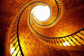
Construction for line segments with lengths whose ratios are the square root of a positive integer

One of the consequences of the Pythagorean theorem is that line segments whose lengths are incommensurable (that is, whose ratio is anirrational number) can be constructed using a straightedge and compass. Pythagoras' theorem enables construction of incommensurable lengths because the hypotenuse of a triangle is related to the sides via the square root operation.

The figure on the right shows how to construct line segments whose lengths are in the ratio of the square root of any positive integer.[30] Each triangle has a side (labeled "1") that is the chosen unit for measurement. In each right triangle, Pythagoras' theorem establishes the length of the hypotenuse in terms of this unit. If a hypotenuse is related to the unit by the square root of a positive integer that is not a perfect square, it is a realization of a length incommensurable with the unit. Examples are 235 . For more detail, see Quadratic irrational.

Incommensurable lengths conflicted with the Pythagorean school's concept of numbers as only whole numbers. The Pythagorean school dealt with proportions by comparison of integer multiples of a common subunit.[31] According to one legend, Hippasus of Metapontum (ca. 470 B.C.) was drowned at sea for making known the existence of the irrational or incommensurable.[32][33]

[edit]Euclidean distance in various coordinate systems

The separation s of two points (r1, θ1)and (r2, θ2) in polar coordinates is given by the law of cosines. Interior angle Δθ = θ1−θ2.

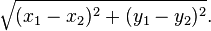
The distance formula in Cartesian coordinates is derived from the Pythagorean theorem.[34] If (x1y1) and (x2y2) are points in the plane, then the distance between them, also called the Euclidean distance, is given by

 sqrt{(x_1-x_2)^2 + (y_1-y_2)^2}.

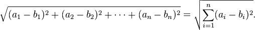
More generally, in Euclidean n-space, the Euclidean distance between two points, A,=,(a_1,a_2,dots,a_n) and B,=,(b_1,b_2,dots,b_n), is defined, by generalization of the Pythagorean theorem, as:

sqrt{(a_1-b_1)^2 + (a_2-b_2)^2 + cdots + (a_n-b_n)^2} = sqrt{sum_{i=1}^n (a_i-b_i)^2}.

If Cartesian coordinates are not used, for example, if polar coordinates are used in two dimensions or, in more general terms, if curvilinear coordinates are used, the formulas expressing the Euclidean distance are more complicated than the Pythagorean theorem, but can be derived from it. A typical example where the straight-line distance between two points is converted to curvilinear coordinates can be found in theapplications of Legendre polynomials in physics. The formulas can be discovered by using Pythagoras' theorem with the equations relating the curvilinear coordinates to Cartesian coordinates. For example, the polar coordinates (rθ) can be introduced as:

 x = r cos theta,  y = r sin theta.,

Then two points with locations (r1θ1) and (r2θ2) are separated by a distance s:

s^2 = (x_1 - x_2)^2 + (y_1-y_2)^2 = (r_1 cos theta_1 -r_2 cos theta_2 )^2 + (r_1 sin theta_1 -r_2 sin theta_2)^2.,

Performing the squares and combining terms, the Pythagorean formula for distance in Cartesian coordinates produces the separation in polar coordinates as:

begin{align}s^2 &= r_1^2 +r_2^2 -2 r_1 r_2 left( cos theta_1 cos theta_2 +sin theta_1 sin theta_2 right)\  &= r_1^2 +r_2^2 -2 r_1 r_2 cos left( theta_1 - theta_2right)\  &=r_1^2 +r_2^2 -2 r_1 r_2 cos Delta theta end{align}  ,

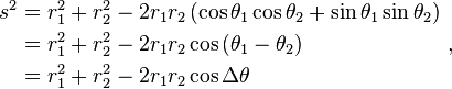
using the trigonometric product-to-sum formulas. This formula is the law of cosines, sometimes called the Generalized Pythagorean Theorem.[35] From this result, for the case where the radii to the two locations are at right angles, the enclosed angle Δθ = π/2, and the form corresponding to Pythagoras' theorem is regained: s^2 = r_1^2 + r_2^2.,  
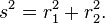
The Pythagorean theorem, valid for right triangles, therefore is a special case of the more general law of cosines, valid for arbitrary triangles.

[edit]Pythagorean trigonometric identity

Similar right triangles showing sine and cosine of angle θ

In a right triangle with sides ab and hypotenuse ctrigonometry determines the sine and cosine of the angle θ between side a and the hypotenuse as:

sin theta = frac{b}{c}, quad cos theta = frac{a}{c}.

From that it follows:

 {cos}^2 theta + {sin}^2 theta = frac{a^2 + b^2}{c^2} = 1,

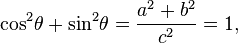
where the last step applies Pythagoras' theorem. This relation between sine and cosine sometimes is called the fundamental Pythagorean trigonometric identity.[36] In similar triangles, the ratios of the sides are the same regardless of the size of the triangles, and depend upon the angles. Consequently, in the figure, the triangle with hypotenuse of unit size has opposite side of size sin θ and adjacent side of size cos θ in units of the hypotenuse.

[edit]Generalizations

[edit]Similar figures on the three sides

Generalization for similar triangles,
green area A + B = blue area C
Pythagoras' theorem using similar right triangles

The Pythagorean theorem was generalized by Euclid in his Elements to extend beyond the areas of squares on the three sides to similar figures:[37]

If one erects similar figures (see Euclidean geometry) on the sides of a right triangle, then the sum of the areas of the two smaller ones equals the area of the larger one.

The basic idea behind this generalization is that the area of a plane figure is proportional to the square of any linear dimension, and in particular is proportional to the square of the length of any side. Thus, if similar figures with areas AB and C are erected on sides with lengths ab andc then:

frac{A}{a^2} = frac{B}{b^2} = frac{C}{c^2}, ,
Rightarrow A + B = frac{a^2}{c^2}C + frac{b^2}{c^2}C, .

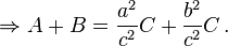
But, by the Pythagorean theorem, a2 + b2 = c2, so A + B = C.

Conversely, if we can prove that A + B = C for three similar figures without using the Pythagorean theorem, then we can work backwards to construct a proof of the theorem. For example, the starting center triangle can be replicated and used as a triangle C on its hypotenuse, and two similar right triangles (A and B ) constructed on the other two sides, formed by dividing the central triangle by its altitude. The sum of the areas of the two smaller triangles therefore is that of the third, thus A + B = C and reversing the above logic leads to the Pythagorean theorem a2 + b2 = c2.

[edit]Law of cosines

The Pythagorean theorem is a special case of the more general theorem relating the lengths of sides in any triangle, the law of cosines:[38]

a^2+b^2-2abcos{theta}=c^2, ,

where θ is the angle between sides a and b.

When θ is 90 degrees, then cosθ = 0, and the formula reduces to the usual Pythagorean theorem.

[edit]Arbitrary triangle

Generalization of Pythagoras' theorem byTâbit ibn Qorra.[39] Lower panel: reflection of triangle ABD (top) to form triangle DBA, similar to triangle ABC (top).

At any selected angle of a general triangle of sides a, b, c, inscribe an isosceles triangle such that the equal angles at its base θ are the same as the selected angle. Suppose the selected angle θ is opposite the side labeled c. Inscribing the isosceles triangle forms triangle ABD with angle θ opposite side a and with side r along c. A second triangle is formed with angle θ opposite side b and a side with length s along c, as shown in the figure. Tâbit ibn Qorra[40] stated that the sides of the three triangles were related as:[41][42]

 a^2 +b^2 =c(r+s)  .

As the angle θ approaches π/2, the base of the isosceles triangle narrows, and lengths r and s overlap less and less. When θ = π/2, ADBbecomes a right triangle, r + s = c, and the original Pythagoras' theorem is regained.

One proof observes that triangle ABC has the same angles as triangle ABD, but in opposite order. (The two triangles share the angle at vertex B, both contain the angle θ, and so also have the same third angle by the triangle postulate.) Consequently, ABC is similar to the reflection ofABD, the triangle DBA in the lower panel. Taking the ratio of sides opposite and adjacent to θ,

frac{c}{a} = frac{a}{r}  .

Likewise, for the reflection of the other triangle,

frac{c}{b} = frac{b}{s}  .

Clearing fractions and adding these two relations:

 cr +cs = a^2 +b^2  ,

the required result.

[edit]General triangles using parallelograms

Generalization for arbitrary triangles,
green area = blue area
Construction for proof of parallelogram generalization

A further generalization applies to triangles that are not right triangles, using parallelograms on the three sides in place of squares.[43] (Squares are a special case, of course.) The upper figure shows that for a scalene triangle, the area of the parallelogram on the longest side is the sum of the areas of the parallelograms on the other two sides, provided the parallelogram on the long side is constructed as indicated (the dimensions labeled with arrows are the same, and determine the sides of the bottom parallelogram). This replacement of squares with parallelograms bears a clear resemblance to the original Pythagoras' theorem, and was considered a generalization by Pappus of Alexandria in 4 A.D.[43]

The lower figure shows the elements of the proof. Focus on the left side of the figure. The left green parallelogram has the same area as the left, blue portion of the bottom parallelogram because both have the same base b and height h. However, the left green parallelogram also has the same area as the left green parallelogram of the upper figure, because they have the same base (the upper left side of the triangle) and the same height normal to that side of the triangle. Repeating the argument for the right side of the figure, the bottom parallelogram has the same area as the sum of the two green parallelograms.

[edit]Complex arithmetic

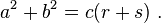
Pythagoras' formula is used to find the distance between two points in the Cartesian coordinate plane, and is valid if all coordinates are real: the distance s between the points (ab) and (cd) is

s = sqrt{(a-c)^2 + (b-d)^2}.

No problem arises with the formula if complex numbers are treated as vectors with real components as in x + i y = (xy). For example, the distance s between 0 + 1i and 1 + 0i becomes the magnitude of the vector (0, 1) − (1, 0) = (−1, 1), or

 s = sqrt{ (-1)^2 +1^2} = sqrt{2}.

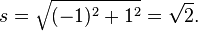
However, a modification of the Pythagorean formula is necessary for a direct treatment of vectors with complex coordinates. The distance between the points with complex coordinates (ab) and (cd); abc, and d all complex; is formulated using absolute values. The distance sis based upon the vector difference (a − cb − d) in the following manner:[44] Let the difference a − c = p + i q, where p is the real part of the difference, q is the imaginary part and i = √(−1). Likewise, let b − d = r + is. Then:

 begin{align} s &= sqrt{(p+iq)overline{(p+iq)} + (r+is)overline{(r+is)}} \   &= sqrt{(p+iq)(p-iq) + (r+is)(r-is)} \   &= sqrt{p^2 + q^2 + r^2 + s^2}, end{align}

where overline{mathit z} is the complex conjugate of mathit z . For example, the distance between the points (ab) = (0, 1) and (cd) = (i, 0) begins with the difference (a − cb − d) = (−i, 1) and would work out as 0 if complex conjugates were not taken. Using the modified formula, the result is

s = sqrt{(-i)cdot(overline{-i}) + 1 cdotoverline{1}}= sqrt{(-i)cdot{i} + 1 cdot{1}} = sqrt{2}. ,

The norm defined by:

|mathbf p | = sqrt{mathbf {p cdot overline{p}}} = sqrt{|p_1|^2 + |p_2|^2 + dots +|p_n|^2}  ,

is a Hermitian dot product.[45]

[edit]Solid geometry

Pythagoras' theorem in three dimensions relates the diagonal AD to the three sides.
A tetrahedron with outward facing right-angle corner

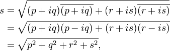
In terms of solid geometry, Pythagoras' theorem can be applied to three dimensions as follows. Consider a rectangular solid as shown in the figure. The length of diagonal BD is found from Pythagoras' theorem as:

 overline{BD}^{,2} = overline{BC}^{,2} + overline{CD}^{,2}  ,

where these three sides form a right triangle. Using horizontal diagonal BD and the vertical edge AB, the length of diagonal AD then is found by a second application of Pythagoras' theorem as:

 overline{AD}^{,2} = overline{AB}^{,2} + overline{BD}^{,2}  ,

or, doing it all in one step:

 overline{AD}^{,2} = overline{AB}^{,2} + overline{BC}^{,2} + overline{CD}^{,2}   .

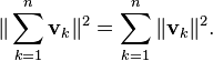
This result is the three-dimensional expression for the magnitude of a vector v (the diagonal AD) in terms of its orthogonal components {vk} (the three mutually perpendicular sides):

|mathbf{v}|^2 = sum_{k=1}^3 |mathbf{v}_k|^2.

This one-step formulation may be viewed as a generalization of Pythagoras' theorem to higher dimensions. However, this result is really just the repeated application of the original Pythagoras' theorem to a succession of right triangles in a sequence of orthogonal planes.

A substantial generalization of the Pythagorean theorem to three dimensions is de Gua's theorem, named for Jean Paul de Gua de Malves: If atetrahedron has a right angle corner (a corner like a cube), then the square of the area of the face opposite the right angle corner is the sum of the squares of the areas of the other three faces. This result can be generalized as in the "n-dimensional Pythagorean theorem":[46]

Let x_1, x_2, ...x_n , be orthogonal vectors in ℝn. Consider the n-dimensional simplex S with vertices 0,x_1 ... x_n,. (Think of the (n−1) dimensional simplex with vertices x_1,...x_n, not including the origin as the "hypotenuse" of S and the remaining (n−1)-dimensional faces of S as its "legs".) Then the square of the volume of the hypotenuse of S is the sum of the squares of the volumes of the n legs.

This statement is illustrated in three dimensions by the tetrahedron in the figure. The "hypotenuse" is the base of the tetrahedron at the back of the figure, and the "legs" are the three sides emanating from the vertex in the foreground. As the depth of the base from the vertex increases, the area of the "legs" increases, while that of the base is fixed. The theorem suggests that when this depth is at the value creating a right vertex, the generalization of Pythagoras' theorem applies. In a different wording:[47]

Given an n-rectangular n-dimensional simplex, the square of the (n − 1)-content of the facet opposing the right vertex will equal the sum of the squares of the (n − 1)-contents of the remaining facets.

[edit]Inner product spaces

Vectors involved in the parallelogram law

The Pythagorean theorem can be generalized to inner product spaces,[48] which are generalizations of the familiar 2-dimensional and 3-dimensional Euclidean spaces. For example, a function may be considered as a vector with infinitely many components in an inner product space, as in functional analysis.[49]

In an inner product space, the concept of perpendicularity is replaced by the concept of orthogonality: two vectors v and w are orthogonal if their inner product  langle mathbf{v} , mathbf{w}rangle  is zero. The inner product is a generalization of the dot product of vectors. The dot product is called the standardinner product or the Euclidean inner product. However, other inner products are possible.[50]

The concept of length is replaced by the concept of the norm ||v|| of a vector v, defined as:[51]

lVert mathbf{v} rVert  equiv  sqrt{langle mathbf{v},mathbf{v}rangle} , .

In this setting, the Pythagorean theorem states that for any two orthogonal vectors v and w of a normed inner product space,

left| mathbf{v} + mathbf{w} right|^2 = left| mathbf{v}  right|^2 +  left| mathbf{w} right|^2  .

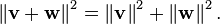
Here the vectors v and w are akin to the sides of a right triangle with hypotenuse given by the vector sum v + w. This form of the Pythagorean theorem is a consequence of the properties of the inner product:

left| mathbf{v} + mathbf{w} right|^2 =langle mathbf{ v+w}, mathbf{ v+w}rangle = langle mathbf{ v}, mathbf{ v}rangle +langle mathbf{ w}, mathbf{ w}rangle +langlemathbf{ v, w }rangle + langlemathbf{ w, v }rangle  = left| mathbf{v}right|^2 + left| mathbf{w}right|^2,

where the inner products of the cross terms are zero by orthogonality.

A further generalization of the Pythagorean theorem in an inner product space to non-orthogonal vectors is the parallelogram law :[51]

2|mathbf v|^2 +2 |mathbf w|^2 = |mathbf {v + w} |^2 +| mathbf{v-w}|^2  ,

which says that twice the sum of the squares of the lengths of the sides of a parallelogram is the sum of the squares of the lengths of the diagonals. Any norm that satisfies this equality is ipso facto a norm corresponding to an inner product.[51]

The identity can be extended to sums of more than two vectors. If v1v2, ..., vn are pairwise-orthogonal vectors in an inner product space, application of the Pythagorean theorem to successive pairs of these vectors (as described for 3-dimensions in the section on solid geometry) results in the equation[52]

|sum_{k=1}^{n}mathbf{v}_k|^2 = sum_{k=1}^n |mathbf{v}_k|^2.

Parseval's identity is a further generalization that considers infinite sums of orthogonal vectors.

[edit]Non-Euclidean geometry

The Pythagorean theorem is derived from the axioms of Euclidean geometry, and in fact, the Pythagorean theorem given above does not hold in a non-Euclidean geometry.[53] (The Pythagorean theorem has been shown, in fact, to be equivalent to Euclid's Parallel (Fifth) Postulate.[54][55]) In other words, in non-Euclidean geometry, the relation between the sides of a triangle must necessarily take a non-Pythagorean form. For example, in spherical geometry, all three sides of the right triangle (say ab, and c) bounding an octant of the unit sphere have length equal to π/2, which violates the Pythagorean theorem because a2 + b2 ≠ c2.

Here two cases of non-Euclidean geometry are considered—spherical geometry and hyperbolic plane geometry; in each case, as in the Euclidean case for non-right triangles, the result replacing the Pythagorean theorem follows from the appropriate law of cosines.

However, the Pythagorean theorem remains true in hyperbolic geometry and elliptic geometry if the condition that the triangle be right is replaced with the condition that two of the angles sum to the third, say A+B = C. The sides are then related as follows: the sum of the areas of the circles with diameters a and b equals the area of the circle with diameter c.[56]

[edit]Spherical geometry

Spherical triangle

For any right triangle on a sphere of radius R (for example, if γ in the figure is a right angle), with sides abc, the relation between the sides takes the form:[57]

 cos left(frac{c}{R}right)=cos left(frac{a}{R}right)cos left(frac{b}{R}right).

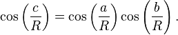
This equation can be derived as a special case of the spherical law of cosines that applies to all spherical triangles:

 cos left(frac{c}{R}right)=cos left(frac{a}{R}right)cos left(frac{b}{R}right) +sinleft(frac{a}{R}right) sinleft(frac{b}{R}right) cos gamma  .

By using the Maclaurin series for the cosine function, cos x ≈ 1 − x2/2, it can be shown that as the radius R approaches infinity and the arguments a/R, b/R and c/R tend to zero, the spherical relation between the sides of a right triangle approaches the form of Pythagoras' theorem. Substituting the approximate quadratic for each of the cosines in the spherical relation for a right triangle:

1-left(frac{c}{R}right)^2= left[1-left(frac{a}{R}right)^2 right]left[1-left(frac{b}{R}right)^2 right] +  mathrm{higher order terms}

Multiplying out the bracketed quantities, Pythagoras' theorem is recovered for large radii R:

left(frac{c}{R}right)^2= left(frac{a}{R}right)^2 + left(frac{b}{R}right)^2 +  mathrm{higher order terms}  ,

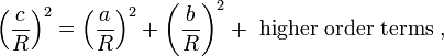
where the higher order terms become negligibly small as R becomes large.

[edit]Hyperbolic geometry

Hyperbolic triangle

For a right triangle in hyperbolic geometry with sides abc and with side c opposite a right angle, the relation between the sides takes the form:[58]

 cosh c=cosh a,cosh b

where cosh is the hyperbolic cosine. This formula is a special form of the hyperbolic law of cosines that applies to all hyperbolic triangles:[59]

cosh c = cosh a  cosh b - sinh a  sinh b  cos gamma  ,

with γ the angle at the vertex opposite the side c.

By using the Maclaurin series for the hyperbolic cosine, cosh x ≈ 1 + x2/2, it can be shown that as a hyperbolic triangle becomes very small (that is, as ab, and c all approach zero), the hyperbolic relation for a right triangle approaches the form of Pythagoras' theorem.

[edit]Differential geometry

Distance between infinitesimally separated points in Cartesian coordinates(top) and polar coordinates (bottom), as given by Pythagoras' theorem

On an infinitesimal level, in three dimensional space, Pythagoras' theorem describes the distance between two infinitesimally separated points as:

ds^2 = dx^2 + dy^2 +dz^2,,

with ds the element of distance and (dxdydz) the components of the vector separating the two points. Such a space is called a Euclidean space. However, a generalization of this expression useful for general coordinates (not just Cartesian) and general spaces (not just Euclidean) takes the form:[60]

ds^2 = sum_{i,j}^n g_{ij}, dx_i, dx_j

where gij is called the metric tensor. It may be a function of position. Such curved spaces include Riemannian geometry as a general example. This formulation also applies to a Euclidean space when using curvilinear coordinates. For example, in polar coordinates:

ds^2 = dr^2 + r^2 dtheta^2  .

[edit]Relation to cross product

The area of a parallelogram as a cross product; vectors a and b identify a plane and a × b is normal to this plane.

Pythagoras' theorem connects two expressions for the magnitude of the cross product.

One approach to defining a vector cross product is to require that it satisfies the equation,[61]

 |mathbf{a} times mathbf{b}|^2  = |mathbf{a}|^2  |mathbf{b}|^2 - (mathbf{a} cdot mathbf{b})^2

which involves the dot product. The right-hand side is called the Gram determinant of a and b, and represents the square of the area of the parallelogram formed by these two vectors. From this requirement along with that of orthogonality of the cross product to its constituents a andb, it follows that, apart from the trivial cases of zero and one dimensions, the cross product is defined only in three and seven dimensions.[62]Using the definition of angle in n-dimensions:[63]

 (mathbf{a cdot b}) = ab  cos theta  ,

this property of the cross product provides its magnitude as:

 |mathbf{ a times b} |^2 =a^2 b^2 left(1 - cos^2 theta right)  .

Through the fundamental Pythagorean trigonometric identity,[36] another form for the magnitude is found:

  |mathbf{ a times b}|=  ab sin theta ,  .

An alternative approach defines the cross product using this expression for its magnitude. Then reversing the above argument, the connection to the dot product:

 |mathbf{a} times mathbf{b}|^2  = |mathbf{a}|^2  |mathbf{b}|^2 - (mathbf{a} cdot mathbf{b})^2 ,

is derived.

[edit]History

The Plimpton 322 tablet records Pythagorean triples from Babylonian times.[7]

There is debate whether the Pythagorean theorem was discovered once, or many times in many places.

The history of the theorem can be divided into four parts: knowledge of Pythagorean triples, knowledge of the relationship among the sides of aright triangle, knowledge of the relationships among adjacent angles, and proofs of the theorem within some deductive system.

Bartel Leendert van der Waerden conjectured that Pythagorean triples were discovered algebraically by the Babylonians.[64] Written between 2000 and 1786 BC, the Middle Kingdom Egyptian papyrus Berlin 6619 includes a problem whose solution is the Pythagorean triple 6:8:10, but the problem does not mention a triangle. The Mesopotamian tablet Plimpton 322, written between 1790 and 1750 BC during the reign ofHammurabi the Great, contains many entries closely related to Pythagorean triples.

In India, the Baudhayana Sulba Sutra, the dates of which are given variously as between the 8th century BC and the 2nd century BC, contains a list of Pythagorean triples discovered algebraically, a statement of the Pythagorean theorem, and a geometrical proof of the Pythagorean theorem for an isosceles right triangle. The Apastamba Sulba Sutra (circa 600 BC) contains a numerical proof of the general Pythagorean theorem, using an area computation. Van der Waerden believes that "it was certainly based on earlier traditions". According to Albert Bŭrk, this is the original proof of the theorem; he further theorizes that Pythagoras visited Arakonam, India, and copied it. Boyer (1991) thinks the elements found in the Śulba-sũtram may be of Mesopotamian derivation.[65]

Geometric proof of the Pythagorean theorem from the Zhou Bi Suan Jing.

With contents known much earlier, but in surviving texts dating from roughly the first century BC, the Chinese text Zhou Bi Suan Jing (周髀算经), (The Arithmetical Classic of the Gnomon and the Circular Paths of Heaven) gives an argument for the Pythagorean theorem for the (3, 4, 5) triangle—in China it is called the "Gougu Theorem" (勾股定理).[66][67] During the Han Dynasty, from 202 BC to 220 AD, Pythagorean triples appear in The Nine Chapters on the Mathematical Art,[68] together with a mention of right triangles.[69] Some believe the theorem arose first in China,[70] where it is alternatively known as the "Shang Gao Theorem" (商高定理),[71] named after the Duke of Zhou's astrologer, and described in the mathematical collection Zhou Bi Suan Jing[72].

Pythagoras, whose dates are commonly given as 569–475 BC, used algebraic methods to construct Pythagorean triples, according toProclus's commentary on Euclid. Proclus, however, wrote between 410 and 485 AD. According to Sir Thomas L. Heath, no specific attribution of the theorem to Pythagoras exists in the surviving Greek literature from the five centuries after Pythagoras lived.[73] However, when authors such as Plutarch and Cicero attributed the theorem to Pythagoras, they did so in a way which suggests that the attribution was widely known and undoubted.[6][74] "Whether this formula is rightly attributed to Pythagoras personally, [...] one can safely assume that it belongs to the very oldest period of Pythagorean mathematics."[33]

Around 400 BC, according to Proclus, Plato gave a method for finding Pythagorean triples that combined algebra and geometry. Circa 300 BC, in Euclid's Elements, the oldest extantaxiomatic proof of the theorem is presented.[75]

[edit]Pop references to the Pythagorean theorem

The Pythagorean theorem has arisen in popular culture in a variety of ways.

  • A verse of the Major-General's Song in the Gilbert and Sullivan comic opera The Pirates of Penzance, "About binomial theorem I'm teeming with a lot o' news, With many cheerful facts about the square of the hypotenuse", makes an oblique reference to the theorem.
  • The Scarecrow of The Wizard of Oz (1939 film) makes a more specific reference to the theorem when he receives his diploma from the Wizard. He immediately exhibits his "knowledge" by reciting a mangled and incorrect version of the theorem: "The sum of the square roots of any two sides of an isosceles triangle is equal to the square root of the remaining side. Oh, joy! Oh, rapture! I've got a brain!" The "knowledge" exhibited by the Scarecrow is incorrect.[76]
  • In 2000, Uganda released a coin with the shape of an isosceles right triangle. The coin's tail has an image of Pythagoras and the equation α2 + β2 = γ2, accompanied with the mention "Pythagoras Millennium".[77] GreeceJapanSan MarinoSierra Leone, and Suriname have issued postage stamps depicting Pythagoras and the Pythagorean theorem.[78]
  • In Neal Stephenson's speculative fiction Anathem, the Pythagorean theorem is referred to as 'the Adrakhonic theorem'. A geometric proof of the theorem is displayed on the side of an alien ship to demonstrate their understanding of mathematics.

[edit]See also

[edit]Notes

  1. a b Judith D. Sally, Paul Sally (2007). "Chapter 3: Pythagorean triples"Roots to research: a vertical development of mathematical problems. American Mathematical Society Bookstore. p. 63.ISBN 0821844032.
  2. ^ Tobias Dantzig (1955). The bequest of the Greeks. Charles Scribner's Sons. p. 97.
  3. ^ (Maor 2007, p. 39)
  4. ^ GJ Allman (1888). Thomas Spencer Baynes. ed. The Encyclopaedia Britannica: A Dictionary of Arts, Sciences, and General Literature, Volume 20 (9th ed.). H.G. Allen. p. 142.
  5. ^ George Johnston Allman (1889). Greek Geometry from Thales to Euclid (Reprinted by Kessinger Publishing LLC 2005 ed.). Hodges, Figgis, & Co. p. 26.ISBN 143260662X. "The discovery of the law of three squares, commonly called the "theorem of Pythagoras" is attributed to him by – amongst others – Vitruvius, Diogenes Laertius, Proclus, and Plutarch ..."
  6. a b (Heath 1921, Vol I, p. 144)
  7. a b Otto Neugebauer (1969). The exact sciences in antiquity (Republication of 1957 Brown University Press 2nd ed.). Courier Dover Publications. p. 36.ISBN 0486223329.. For a different view, see Dick Teresi (2003). Lost Discoveries: The Ancient Roots of Modern Science. Simon and Schuster. p. 52.ISBN 074324379X., where the speculation is made that the first column of a tablet 322 in the Plimpton collectionsupports a Babylonian knowledge of some elements of trigonometry. That notion is pretty much laid to rest byEleanor Robson (2002). "Words and Pictures: New Light on Plimpton 322"The American Mathematical Monthly(Mathematical Association of America) 109 (2): 105–120.doi:10.2307/2695324. See also pdf file. The accepted view today is that the Babylonians had no awareness of trigonometric functions. See Abdulrahman A. Abdulaziz (2010). "The Plimpton 322 Tablet and the Babylonian Method of Generating Pythagorean Triples"ArXiv preprint. §2, page 7.
  8. ^ Mario Livio (2003). The golden ratio: the story of phi, the world's most astonishing number. Random House, Inc. p. 25. ISBN 0767908163.
  9. ^ (Loomis 1968)
  10. ^ (Maor 2007, p. 39) page 39
  11. a b Stephen W. Hawking (2005). God created the integers: the mathematical breakthroughs that changed history. Philadelphia: Running Press Book Publishers. p. 12. ISBN 0762419229.
  12. ^ See for example Mike May S.J., Pythagorean theorem by shear mapping, Saint Louis University website Java applet
  13. ^ Jan Gullberg (1997). Mathematics: from the birth of numbers. W. W. Norton & Company. p. 435.ISBN 039304002X.
  14. ^ Elements 1.47 by Euclid. Retrieved 19 December 2006.
  15. ^ Euclid's Elements, Book I, Proposition 47: web page version using Java applets from Euclid's Elements by Prof. David E. Joyce, Clark University
  16. ^ The proof by Pythagoras probably was not a general one, as the theory of proportions was developed only two centuries after Pythagoras; see (Maor 2007, p. 25) page 25
  17. ^ (Loomis 1968, Geometric proof 22 and Figure 123, page= 113)
  18. ^ Alexander Bogomolny. "Pythagorean Theorem, proof number 10"Cut the Knot. Retrieved 27 February 2010.
  19. ^ Alexander Bogomolny. "Cut-the-knot.org: Pythagorean theorem and its many proofs, Proof #3"Cut the Knot. Retrieved 4 November 2010.
  20. ^ Alexander Bogomolny. "Cut-the-knot.org: Pythagorean theorem and its many proofs, Proof #4"Cut the Knot. Retrieved 4 November 2010.
  21. ^ Published in a weekly mathematics column: James A Garfield (1876). The New England Journal of Education 3: 161. as noted in William Dunham (1997). The mathematical universe: An alphabetical journey through the great proofs, problems, and personalities. Wiley. p. 96. ISBN 0471176613. and in A calendar of mathematical dates: April 1, 1876 by V. Frederick Rickey
  22. ^ Prof. David Lantz' animation from his web site of animated proofs
  23. a b Mike Staring (1996). "The Pythagorean proposition: A proof by means of calculus"Mathematics Magazine(Mathematical Association of America) 69 (February): 45–46. doi:10.2307/2691395.
    (An abbreviated version of this proof is in the second half of Proof #40 at Bogomolny, Alexander. "Pythagorean Theorem"Interactive Mathematics Miscellany and Puzzles. Alexander Bogomolny. Retrieved 2010-05-09.Archived version May 8, 2010.)
  24. ^ Proof #40 also summarizes a differential proof by Michael Hardy: "Pythagoras Made Difficult". Mathematical Intelligencer10 (3), p. 31, 1988. Although not listed in this journal's table of contents and without a doi, this article can be found at the end of the unrelated article byBruce C. Berndt (1988). "Ramanujan—100 years old (fashioned) or 100 years new (fangled)?". The Mathematical Intelligencer 10: 24.doi:10.1007/BF03026638.
  25. ^ From the figure, it is evident that point D lies inside the circle of radius c, which is why AD is larger than Δc. That fact is rigorously established by noting side CD of right triangle CDP must be less than c because it is necessarily less than the hypotenuse CP of CDP. Consequently, point D definitely is inside the circle of radius c. Similarly, point Q must lie inside the circle of radius c + Δc because CQ must be less than the hypotenuse CA of right triangle CQA, of length c + Δc. The theorem that the hypotenuse of a right triangle is longer than either of its sides does not require Pythagoras' theorem, so the derivation is not simply circular. However, that theorem in turn does require the triangle postulate, equivalent to Euclid's postulate of parallel lines.
  26. ^ Judith D. Sally, Paul Sally (2007-12-21). "Theorem 2.4 (Converse of the Pythagorean Theorem)."Cited work. p. 62. ISBN 0821844032.
  27. ^ Euclid's Elements, Book I, Proposition 48 From D.E. Joyce's web page at Clark University
  28. ^ Ernest Julius Wilczynski, Herbert Ellsworth Slaught (1914). "Theorem 1 and Theorem 2"Plane trigonometry and applications. Allyn and Bacon. p. 85.
  29. ^ "Dijkstra's generalization" (PDF).
  30. ^ Henry Law (1853). "Corollary 5 of Proposition XLVII,Pythagoras' Theorem"The elements of Euclid: with many additional propositions, & explanatory notes to which is prefixed an introductory essay on logic. John Weale. p. 49.
  31. ^ Shaughan Lavine (1994). Understanding the infinite. Harvard University Press. p. 13. ISBN 0674920961.
  32. ^ (Heath 1921, Vol I, pp. 65); Hippasus was on a voyage at the time, and his fellows cast him overboard. SeeJames R. Choike (1980). "The pentagram and the discovery of an irrational number". The College Mathematics Journal 11: 312–316.
  33. a b A careful discussion of Hippasus' contributions is found in Kurt Von Fritz (Apr., 1945). "The Discovery of Incommensurability by Hippasus of Metapontum"The Annals of Mathematics, Second Series (Annals of Mathematics) 46 (2): 242–264.
  34. ^ Jon Orwant, Jarkko Hietaniemi, John Macdonald (1999). "Euclidean distance"Mastering algorithms with Perl. O'Reilly Media, Inc. p. 426. ISBN 1565923987.
  35. ^ Wentworth, George (2009). Plane Trigonometry and Tables. BiblioBazaar, LLC. p. 116. ISBN 1-103-07998-0Exercises, page 116
  36. a b Lawrence S. Leff (2005). PreCalculus the Easy Way (7th ed.). Barron's Educational Series. p. 296.ISBN 0764128922.
  37. ^ Euclid's Elements: Book VI, Proposition VI 31: "In right-angled triangles the figure on the side subtending the right angle is equal to the similar and similarly described figures on the sides containing the right angle."
  38. ^ Lawrence S. Leff (2005-05-01). cited work. Barron's Educational Series. p. 326. ISBN 0764128922.
  39. ^ Howard Whitley Eves (1983). "§4.8:...generalization of Pythagorean theorem"Great moments in mathematics (before 1650). Mathematical Association of America. p. 41. ISBN 0883853108.
  40. ^ Tâbit ibn Qorra (full name Thābit ibn Qurra ibn Marwan Al-Ṣābiʾ al-Ḥarrānī) ( 826–901 AD) was a physician living in Baghdad who wrote extensively on Euclid's Elements and other mathematical subjects.
  41. ^ Aydin Sayili (Mar. 1960). "Thâbit ibn Qurra's Generalization of the Pythagorean Theorem"Isis 51(1): 35–37. doi:10.1086/348837.
  42. ^ Judith D. Sally, Paul Sally (2007-12-21). "Exercise 2.10 (ii)"Cited work. p. 62. ISBN 0821844032.
  43. a b For the details of such a construction, see George Jennings (1997). "Figure 1.32: The generalized Pythagorean theorem"Modern geometry with applications: with 150 figures (3rd ed.). Springer. p. 23.ISBN 038794222X.
  44. ^ Arlen Brown, Carl M. Pearcy (1995). "Item C: Norm for an arbitrary n-tuple ..."An introduction to analysis. Springer. p. 124. ISBN 0387943692. See also pages 47–50.
  45. ^ Alfred Gray, Elsa Abbena, Simon Salamon (2006).Modern differential geometry of curves and surfaces with Mathematica (3rd ed.). CRC Press. p. 194.ISBN 1584884487.
  46. ^ Rajendra Bhatia (1997). Matrix analysis. Springer. p. 21. ISBN 0387948465.
  47. ^ For an extended discussion of this generalization, see, for example, Willie W. Wong 2002, A generalized n-dimensional Pythagorean theorem.
  48. ^ Ferdinand van der Heijden, Dick de Ridder (2004).Classification, parameter estimation, and state estimation. Wiley. p. 357. ISBN 0470090138.
  49. ^ Qun Lin, Jiafu Lin (2006). Finite element methods: accuracy and improvement. Elsevier. p. 23.ISBN 7030166566.
  50. ^ Howard Anton, Chris Rorres (2010). Elementary Linear Algebra: Applications Version (10th ed.). Wiley. p. 336.ISBN 0470432055.
  51. a b c Karen Saxe (2002). "Theorem 1.2"Beginning functional analysis. Springer. p. 7. ISBN 0387952241.
  52. ^ Douglas, Ronald G. (1998). Banach Algebra Techniques in Operator Theory, 2nd edition. New York, New York: Springer-Verlag New York, Inc. pp. 60–1.ISBN 978-0387983776.
  53. ^ Stephen W. Hawking (2005). cited work. p. 4.ISBN 0762419229.
  54. ^ Eric W. Weisstein (2003). CRC concise encyclopedia of mathematics (2nd ed.). p. 2147. ISBN 1584883472. "The parallel postulate is equivalent to the Equidistance postulatePlayfair axiomProclus axiom, the Triangle postulate and the Pythagorean theorem."
  55. ^ Alexander R. Pruss (2006). The principle of sufficient reason: a reassessment. Cambridge University Press. p. 11. ISBN 052185959X. "We could include...the parallel postulate and derive the Pythagorean theorem. Or we could instead make the Pythagorean theorem among the other axioms and derive the parallel postulate."
  56. ^ Victor Pambuccian (December 2010). "Maria Teresa Calapso's Hyperbolic Pythagorean Theorem". The Mathematical Intelligencer 32 (4): 2. doi:10.1007/s00283-010-9169-0.
  57. ^ Barrett O'Neill (2006). "Exercise 4"Elementary differential geometry (2nd ed.). Academic Press. p. 441.ISBN 0120887355.
  58. ^ Saul Stahl (1993). "Theorem 8.3"The Poincaré half-plane: a gateway to modern geometry. Jones & Bartlett Learning. p. 122. ISBN 086720298X.
  59. ^ Jane Gilman (1995). "Hyperbolic triangles"Two-generator discrete subgroups of PSL(2,R). American Mathematical Society Bookstore. ISBN 0821803611.
  60. ^ Tai L. Chow (2000). Mathematical methods for physicists: a concise introduction. Cambridge University Press. p. 52. ISBN 0521655447.
  61. ^ WS Massey (Dec. 1983). "Cross products of vectors in higher dimensional Euclidean spaces"The American Mathematical Monthly (Mathematical Association of America) 90 (10): 697–701. doi:10.2307/2323537.
  62. ^ Although a cross-product involving n−1 vectors can be found in n-dimensions, a cross-product involving only two vectors can be found only in 3-dimensions and in 7-dimensions. See Pertti Lounesto (2001). "§7.4 Cross product of two vectors"Clifford algebras and spinors(2nd ed.). Cambridge University Press. p. 96.ISBN 0521005515.
  63. ^ Francis Begnaud Hildebrand (1992). Methods of applied mathematics (Reprint of Prentice-Hall 1965 2nd ed.). Courier Dover Publications. p. 24.ISBN 0486670023.
  64. ^ (van_der_Waerden 1983, p. 5) See also Frank Swetz, T. I. Kao (1977). Was Pythagoras Chinese?: An examination of right triangle theory in ancient China. Penn State Press. p. 12. ISBN 0271012382.
  65. ^ Carl Benjamin Boyer (1968). "China and India"A history of mathematics. Wiley. p. 229. "we find rules for the construction of right angles by means of triples of cords the lengths of which form Pythagorean triages, such as 3, 4, and 5, or 5, 12, and 13, or 8, 15, and 17, or 12, 35, and 37. However all of these triads are easily derived from the old Babylonian rule; hence, Mesopotamian influence in the Sulvasũtras is not unlikely. Aspastamba knew that the square on the diagonal of a rectangle is equal to the sum of the squares on the two adjacent sides, but this form of the Pythagorean theorem also may have been derived from Mesopotamia. [...] So conjectural are the origin and period of the Sulvasũtras that we cannot tell whether or not the rules are related to early Egyptian surveying or to the later Greek problem of altar doubling. They are variously dated within an interval of almost a thousand years stretching from the eighth century B.C. to the second century of our era."; See also Carl B. Boyer , Uta C. Merzbach (2010). A History of Mathematics (3rd ed.). Wiley. ISBN 0470525487.
  66. ^ Robert P. Crease (2008). The great equations: breakthroughs in science from Pythagoras to Heisenberg. W W Norton & Co.. p. 25. ISBN 039306204X.
  67. ^ A rather extensive discussion of the origins of the various texts in the Zhou Bi is provided by Christopher Cullen (2007). Astronomy and Mathematics in Ancient China: The 'Zhou Bi Suan Jing'. Cambridge University Press. pp. 139 fISBN 0521035376.
  68. ^ This work is a compilation of 246 problems, some of which survived the book burning of 213 BC, and was put in final form before 100 AD. It was extensively commented upon by Liu Hui in 263 AD. Philip D Straffin, Jr. (2004). "Liu Hui and the first golden age of Chinese mathematics". In Marlow Anderson, Victor J. Katz, Robin J. Wilson. Sherlock Holmes in Babylon: and other tales of mathematical history. Mathematical Association of America. pp. 69 ffISBN 0883855461. See particularly §3: Nine chapters on the mathematical art, pps. 71 ff.
  69. ^ Kangshen Shen, John N. Crossley, Anthony Wah-Cheung Lun (1999). The nine chapters on the mathematical art: companion and commentary. Oxford University Press. p. 488. ISBN 0198539363.
  70. ^ In particular, Li Jimin; see Centaurus, Volume 39. Copenhagen: Munksgaard. 1997. pp. 193 & 205.
  71. ^ Chen, Cheng-Yih (1996). "§3.3.4 Chén Zǐ's formula and the Chóng-Chã method; Figure 40"Early Chinese work in natural science: a re-examination of the physics of motion, acoustics, astronomy and scientific thoughts. Hong Kong University Press. p. 142. ISBN 962209385X.
  72. ^ Wen-tsün Wu (2008). "The Gougu theorem".Selected works of Wen-tsün Wu. World Scientific. p. 158.ISBN 9812791078.
  73. ^ (Euclid 1956, p. 351) page 351
  74. ^ An extensive discussion of the historical evidence is provided in (Euclid 1956, p. 351) page=351
  75. ^ Asger Aaboe (1997). Episodes from the early history of mathematics. Mathematical Association of America. p. 51. ISBN 0883856131. "...it is not until Euclid that we find a logical sequence of general theorems with proper proofs."
  76. ^ "The Scarecrow's Formula"Internet Movie Data Base. Retrieved 2010-05-12.
  77. ^ "Le Saviez-vous ?".
  78. ^ Miller, Jeff (2007-08-03). "Images of Mathematicians on Postage Stamps". Retrieved 2010-07-18.

[edit]References

[edit]External links

Contents

 [hide]
Proof by rearrangement of four identical right triangles
Animation showing another proof by rearrangement[18]
Proof using an elaborate rearrangement

19:40 Publié dans Pythagorean theorem | Lien permanent | Commentaires (0) | |  del.icio.us | | Digg! Digg |  Facebook

Conseils de méthode pour l'épreuve de maths

Conseils de méthode pour l'épreuve de maths

> Conseils en français 
> Conseils en histoire-géo.

Quatres règles impératives

 
Avant de démarrer un calcul ou de commencer à rédiger vos réponses, il convient de respecter certaines règles élémentaires pour éviter de partir sur une fausse piste : 
• Règle 1 : Lire correctement tout l'énoncé de l'exercice. 
• Règle 2 : S'assurer qu'on a compris tout le vocabulaire rencontré dans le texte, et définir clairement la question posée. 
• Règle 3 : Regarder si l'exercice possède des questions dépendant les unes des autres (« exercice à tiroirs »). Alors vous trouverez dans certaines questions des éléments de réponse relatifs aux questions précédentes. 
• Règle 4 : Faire immédiatement une figure dans le cas d'un exercice de géométrie. Vous devez ainsi rendre concret le texte proposé. Attention, le dessin doit être très clair et ne pas correspondre à un cas particulier si ce cas n'est pas envisagé dans l'énoncé. N'hésitez pas à utiliser différentes couleurs pour la composition du schéma. 


Deux conseils complémentaires

• La rédaction de vos réponses doit être claire et rigoureuse . Il est indispensable de rappeler précisément les théorèmes que vous utilisez. 
Un raisonnement en mathématiques doit comprendre des enchaînements logiques et ne doit pas être une suite de lignes de calculs sans liens entre elles. 

• Enfin, n'oubliez pas de mettre en évidence vos réponses (en les encadrant par exemple) et de faire tous vos schémas et graphes sur des feuilles différentes de celles utilisées pour rédiger votre devoir.


Source : http://www.annabrevet.com/methodologie_maths.php

Livres Annabrevet

19:38 | Lien permanent | Commentaires (0) | |  del.icio.us | | Digg! Digg |  Facebook

Table of mathematical symbols

Table of mathematical symbols

From Wikipedia, the free encyclopedia Source : 

Common symbols

This is a listing of common symbols found within all branches of mathematics. Each symbol is listed in both HTML, which depends on appropriate fonts to be installed, and in TEX, as an image.

See also

Variations

In mathematics written in Arabic, some symbols may be reversed to make right-to-left reading easier. [11]

References

  1. ^ Rónyai, Lajos (1998), Algoritmusok(Algorithms), TYPOTEX, ISBN 963-9132-16-0
  2. ^ Berman, Kenneth A; Paul, Jerome L. (2005), Algorithms: Sequential, Parallel, and DistributedBoston: Course Technology, p. 822, ISBN 0-534-42057-5
  3. ^ Nielsen, Michael A; Chuang, Isaac L (2000), Quantum Computation and Quantum InformationNew YorkCambridge University Press, p. 66, ISBN 0-521-63503-9OCLC 43641333
  4. ^ Copi, Irving M.Cohen, Carl (1990) [1953], "Chapter 8.3: Conditional Statements and Material Implication", Introduction to Logic (8th ed.), New YorkMacmillan, pp. 268–269,ISBN 0023250356LCCN 89-37742
  5. a b c d e Goldrei, Derek (1996), Classic Set Theory, London: Chapman and Hall, p. 3, ISBN 0-412-60610-0
  6. a b c d Goldrei, Derek (1996), Classic Set Theory, London: Chapman and Hall, p. 4, ISBN 0-412-60610-0
  7. ^ Goldrei, Derek (1996), Classic Set Theory, London: Chapman and Hall, p. 5, ISBN 0-412-60610-0
  8. ^ Nielsen, Michael A; Chuang, Isaac L (2000), Quantum Computation and Quantum InformationNew YorkCambridge University Press, p. 62, ISBN 0-521-63503-9OCLC 43641333
  9. ^ Nielsen, Michael A; Chuang, Isaac L (2000), Quantum Computation and Quantum InformationNew YorkCambridge University Press, pp. 69–70, ISBN 0-521-63503-9OCLC 43641333
  10. ^ Nielsen, Michael A; Chuang, Isaac L (2000), Quantum Computation and Quantum InformationNew YorkCambridge University Press, pp. 71–72, ISBN 0-521-63503-9OCLC 43641333
  11. ^ M. Benatia, A. Lazrik, and K. Sami, "Arabic mathematical symbols in Unicode", 27th Internationalization and Unicode Conference, 2005.

External links

Some Unicode charts of mathematical operators:

Some Unicode cross-references:

Contents

 [hide]
Symbol
in HTML
Symbol
in TEX
NameExplanationExamples
Read as
Category
= !,
is equal to; equals
everywhere
x = y means x and y represent the same thing or value. 2 = 2
1 + 1 = 2
ne !,
is not equal to; does not equal
everywhere
x ≠ y means that x and y do not represent the same thing or value.

(The forms !=, /= or <> are generally used in programming languages where ease of typing and use of ASCII text is preferred.)
2 + 2 ≠ 5
< !,

> !,
is less than, is greater than
x < y means x is less than y.

x > y means x is greater than y.
3 < 4
5 > 4
is a proper subgroup of
H < G means H is a proper subgroup of G. 5Z < Z
A3  < S3
ll !,

gg !,
is much less than, is much greater than
x ≪ y means x is much less than y.

x ≫ y means x is much greater than y.
0.003 ≪ 1000000
asymptotic comparison
is of smaller order than, is of greater order than
f ≪ g means the growth of f is asymptotically bounded by g.

(This is I. M. Vinogradov's notation. Another notation is the Big O notation, which looks like f = O(g).)
x ≪ ex
le !,

ge !,
is less than or equal to, is greater than or equal to
x ≤ y means x is less than or equal to y.

x ≥ y means x is greater than or equal to y.

(The forms <= and >= are generally used in programming languages where ease of typing and use of ASCII text is preferred.)
3 ≤ 4 and 5 ≤ 5
5 ≥ 4 and 5 ≥ 5
is a subgroup of
H ≤ G means H is a subgroup of G. Z ≤ Z
A3  ≤ S3
is reducible to
A ≤ B means the problem A can be reduced to the problem B. Subscripts can be added to the ≤ to indicate what kind of reduction. If
exists f in F mbox{ . } forall x in mathbb{N} mbox{ . } x in A Leftrightarrow f(x) in B

then

A leq_{F} B
prec !,
is Karp reducible to; is polynomial-time many-one reducible to
L1 ≺ L2 means that the problem L1 is Karp reducible to L2.[1] If L1 ≺ L2 and L2 ∈ P, then L1 ∈ P.
propto !,
is proportional to; varies as
everywhere
y ∝ x means that y = kx for some constant k. if y = 2x, then y ∝ x.
is Karp reducible to; is polynomial-time many-one reducible to
A ∝ B means the problem A can be polynomially reduced to the problem B. If L1 ∝ L2 and L2 ∈ P, then L1 ∈ P.
+ !,
plus; add
4 + 6 means the sum of 4 and 6. 2 + 7 = 9
the disjoint union of ... and ...
A1 + A2 means the disjoint union of sets A1 and A2. A1 = {3, 4, 5, 6} ∧ A2 = {7, 8, 9, 10} ⇒
A1 + A2 = {(3,1), (4,1), (5,1), (6,1), (7,2), (8,2), (9,2), (10,2)}
- !,
minus; take; subtract
9 − 4 means the subtraction of 4 from 9. 8 − 3 = 5
negative; minus; the opposite of
−3 means the negative of the number 3. −(−5) = 5
minus; without
A − B means the set that contains all the elements of A that are not in B.

(∖ can also be used for set-theoretic complement as described below.)
{1,2,4} − {1,3,4}  =  {2}
times !,
times; multiplied by
3 × 4 means the multiplication of 3 by 4.

(The symbol * is generally used in programming languages, where ease of typing and use of ASCII text is preferred.)
7 × 8 = 56
the Cartesian product of ... and ...; the direct product of ... and ...
X×Y means the set of all ordered pairs with the first element of each pair selected from X and the second element selected from Y. {1,2} × {3,4} = {(1,3),(1,4),(2,3),(2,4)}
cross
u × v means the cross product of vectors u and v (1,2,5) × (3,4,−1) =
(−22, 16, − 2)
the group of units of
R× consists of the set of units of the ring R, along with the operation of multiplication.

This may also be written Ras described below, or U(R).
begin{align} (mathbb{Z} / 5mathbb{Z})^times & = { [1], [2], [3], [4] } \ & cong C_4 \ end{align}
cdot !,
times; multiplied by
3 · 4 means the multiplication of 3 by 4. 7 · 8 = 56
dot
u · v means the dot product of vectors u and v (1,2,5) · (3,4,−1) = 6
div !,

/ !,
divided by; over
6 ÷ 3 or 6 ⁄ 3 means the division of 6 by 3. 2 ÷ 4 = .5

12 ⁄ 4 = 3
mod
G / H means the quotient of group G modulo its subgroup H. {0, a, 2abb+ab+2a} / {0, b} = {{0, b}, {ab+a}, {2ab+2a}}
quotient set
mod
A/~ means the set of all ~ equivalence classes in A. If we define ~ by x ~ y ⇔ x − y ∈ , then
/~ = {x + n : n ∈  : x ∈ (0,1]}
pm !,
plus or minus
6 ± 3 means both 6 + 3 and 6 − 3. The equation x = 5 ± √4, has two solutions, x = 7 and x = 3.
plus or minus
10 ± 2 or equivalently 10 ± 20% means the range from 10 − 2 to 10 + 2. If a = 100 ± 1 mm, then a ≥ 99 mm and a ≤ 101 mm.
mp !,
minus or plus
6 ± (3  5) means both 6 + (3 − 5) and 6 − (3 + 5). cos(x ± y) = cos(x) cos(y sin(x) sin(y).
surd !,

sqrt{ } !,
the (principal) square root of
sqrt{x} means the nonnegative number whose square is x. sqrt{4}=2
the (complex) square root of
if z=r,exp(iphi) is represented in polar coordinates with -pi < phi le pi, then sqrt{z} = sqrt{r} exp(i phi/2). sqrt{-1}=i
|…|
| ldots | !,
absolute value or modulus
absolute value of; modulus of
|x| means the distance along the real line (or across the complex plane) between x and zero. |3| = 3

|–5| = |5| = 5

i | = 1

| 3 + 4i | = 5
Euclidean norm or Euclidean length or magnitude
Euclidean norm of
|x| means the (Euclidean) length of vector x. For x = (3,-4)
|textbf{x}| = sqrt{3^2 + (-4)^2} = 5
determinant of
|A| means the determinant of the matrix A begin{vmatrix}  1&2 \  2&4 \ end{vmatrix} = 0
cardinality of; size of; order of
|X| means the cardinality of the set X.

(# may be used instead as described below.)
|{3, 5, 7, 9}| = 4.
||…||
| ldots | !,
norm of; length of
|| x || means the norm of the element x of a normed vector space.[3] || x  + y || ≤  || x ||  +  || y ||
nearest integer to
||x|| means the nearest integer to x.

(This may also be written [x], ⌊x⌉, nint(xor Round(x).)
||1|| = 1, ||1.6|| = 2, ||−2.4|| = −2, ||3.49|| = 3


mid !,

 nmid !,
divides
a|b means a divides b.
ab means a does not divide b.

(This symbol can be difficult to type, and its negation is rare, so a regular but slightly shorter vertical bar | character can be used.)
Since 15 = 3×5, it is true that 3|15 and 5|15.
given
P(A|B) means the probability of the event a occurring given that boccurs. if X is a uniformly random day of the year P(X is May 25 | X is in May) = 1/31
restriction of … to …; restricted to
f|A means the function f restricted to the set A, that is, it is the function with domain A ∩ dom(f) that agrees with f. The function f : R → R defined by f(x) = x2 is not injective, but f|R+is injective.
such that
such that; so that
everywhere
| means “such that”, see ":" (described below). S = {(x,y) | 0 < y < f(x)}
The set of (x,y) such that y is greater than 0 and less than f(x).
||
| !,
is parallel to
x || y means x is parallel to y. If l || m and m ⊥ n then l ⊥ n.
is incomparable to
x || y means x is incomparable to y. {1,2} || {2,3} under set containment.
exactly divides
pa || n means pa exactly divides n (i.e. pa divides n but pa+1 does not). 23 || 360.
# !,
cardinality of; size of; order of
#X means the cardinality of the set X.

(|…| may be used instead as described above.)
#{4, 6, 8} = 3
connected sum of; knot sum of; knot composition of
A#B is the connected sum of the manifolds A and B. If A and Bare knots, then this denotes the knot sum, which has a slightly stronger condition. A#Sm is homeomorphic to A, for any manifold A, and the sphereSm.
aleph !,
aleph
α represents an infinite cardinality (specifically, the α-th one, where α is an ordinal). |ℕ| = ℵ0, which is called aleph-null.
beth !,
beth
α represents an infinite cardinality (similar to ℵ, but ℶ does not necessarily index all of the numbers indexed by ℵ. ). beth_1 = |P(mathbb{N})| = 2^{aleph_0}.

19:34 | Lien permanent | Commentaires (0) | |  del.icio.us | | Digg! Digg |  Facebook

Relational Algebra Translator

Relational Algebra Translator


Este software fue desarrollado como proyecto de investigación a cardo del docente M.Sc. Johnny Villalobos Murillo y programado por el estudiante Steven Brenes Chavarría (sbrenesms@gmail.com) de la Universidad Nacional de Costa Rica. El sistema "Relational Algebra Translator (RAT)" cuenta con las siguientes características:


Versión 2.x


   Arboles de parser

   Operadores nuevos (RO, asignación)

   Mejora en la interfaz 


Versión 1.x


   Analizador lexicográfico

   Analizador semántico

   Generador de arboles de parser

   Traductor al SQL

   Conexiones a Sistemas Gestores de Bases de Datos

   Ejecutar instrucciones SQL


RAT permite al estudiante escribir sentencias en algebra relacional las cuales son traducidas al lenguaje SQL con el propósito de verificar las sintaxis correcta de estas expresiones. RAT permite además establecer conexiones a bases de datos relacionales como: Oracle, MySQL, SQL Server, PostGres, Access por citar algunas, mediante una opción de conexión, para que el estudiante pueda obtener visualmente los resultados de sus consultas en forma de tablas.

Regresar al sitio del laboratorio de bases de datos


This software was developed as a research project on teaching M.Sc. Johnny Villalobos Murillo and scheduled by the student Steven Chaves Brenes (sbrenesms@gmail.com) National University of Costa Rica. The system "Relational Algebra Translator (RAT)" has the following characteristics:

Version 2.x


   Tree parser
   New operators (RO, assignment)
   Improved interface

Version 1.x

   Lexical analyzer
   Semantic analyzer
   Parser generator trees
   SQL translator
   Connections Systems Database Managers
   Execute SQL statements

RAT allows students to write statements in relational algebra which are translated to SQL language in order to verify the correct syntax for these expressions. RAT also allows connections to relational databases such as Oracle, MySQL, SQL Server, Postgres, Access to name a few, through a connection option for the student to visually obtain the results of their consultations in the form of tables.


Source : http://www.slinfo.una.ac.cr/rat/rat.html

19:30 | Lien permanent | Commentaires (0) | |  del.icio.us | | Digg! Digg |  Facebook

Algèbre relationnelle

Algèbre relationnelle

Page d'aide sur l'homonymie Pour les articles homonymes, voir Algèbre (homonymie).

L'algèbre relationnelle est une théorie mathématique proche de la théorie des ensembles qui définit des opérations qui peuvent être effectuées sur des relations - des matricescontenant un ensemble de nuplets.

Au sujet de l'algèbre relationnelle[modifier]

L'algèbre relationnelle a été inventée en 1970 par Edgar Frank Codd, le directeur de recherche du centre IBM de San José. Cet algèbre est constituée d'un ensemble d'opérations formelles sur les relations. Les opérations relationnelles permettent de créer une nouvelle relation (table) à partir d'opérations élémentaires sur d'autres tables (par exemple l'union, l'intersection, ou encore la différence).

Les principes de l'algèbre relationnelle sont beaucoup utilisés de nos jours par les SGBD pour la gestion des bases de données informatiques comme le SQLDBase, etc.

Cependant, les bases de données relationnelles ne fonctionnent pas tout à fait selon les règles ensemblistes de l'algèbre relationnelle. En effet, si l'on ne définit pas de clé primaire, il est possible d'insérer plusieurs lignes identiques dans une table, ce qui d'un point de vue ensembliste n'a pas de sens : un élément fait partie ou ne fait pas partie d'un ensemble. Si l'on veut appliquer strictement les règles des ensembles, il faut vérifier à chaque ajout dans une table que les lignes ne sont pas déjà présentes.

Eléments du modèle relationnel[modifier]

Objets précis du modèle[modifier]

Il s'agit ici de déterminer des Domaines (i.e., type atomique) :

  • Numérique : entier ou réel (SQL : Int, Float, etc.).
  • Chaîne de caractères (SQL : Char(20), VarChar(32), etc.).
  • Date (SQL : DATE, TIME, YEAR, etc.).
  • Type énuméré.

Relation ou Table[modifier]

Une relation (au sens du modèle de Codd) est constituée de deux choses :

  1. Un Schéma : Le format de la table. Le schéma est fixé.
  2. Une Extension : Le contenu de la table, qui est un ensemble de n-uplets dont l'ordre n'a pas d'importance.

Exemple :

Schéma :

{Cle: INT, Nom: VarChar(20), Email: VarChar(20)}

Extension :

{
 {Cle: 1, Nom: "Edgar", Email: "edgar@xxxxx.xx"}
 {Cle: 2, Nom: "Frank", Email: "Frank@xxxxx.xx"}
 ...
}

Requêtes en Algèbre relationnelle[modifier]

Définir un ensemble d'opérations élémentaires permettant, par combinaison éventuelle, d'obtenir les résultats escomptés.

La sélection (ou restriction) :

  • Notation : sigma_{F}( R ),
  • Données : Une relation R, et une formule F, formée d'une combinaison de comparaisons et de connecteurs logiques.
  • Résultat : sigma_{F}( R ) = { r in R : r, satisfait la condition donnée par F },
  • Équivalent SQL : WHERE

La projection :

  • Notation : pi_{A}( R ),
  • Données : Une relation R, et un ensemble d'attributs A, de R,.
  • Résultat : pi_{A}( R ),, qui est la Relation R, où on ne considère que les attributs de A,
  • Équivalent SQL : SELECT

Rebaptiser :

  • Notation : rho_{a/b}(R),
  • Données : Une relation R, et un attribut b, de R,.
  • Résultat : rho_{a/b}(R),, qui est la Relation R, avec b, rebaptisé a,
  • Équivalent SQL : AS

Opérateurs ensemblistes[modifier]

L'algèbre relationnelle possède les opérations usuelles sur les ensembles.

Soient R(A), et S(B), deux relations ayant pour ensembles d'attributs respectifs A, et B,:

Ainsi, tout n-uplet r in R , se décompose en deux n-uplets r=(t,s),,
avec t=(t_1, ..., t_m), de schéma X={x_1, ..., x_m}, et
s=(s_1, ..., s_p), de schéma y={y_1, ..., y_p},.
et retourne la table de schéma X, tel que R/S={t: forall s in S,  (t,s) in R},
La division revient à donner “tous les x tels que pour tout y ...”

Exemples[modifier]

  • Relations de la base exemple :

Table Touristes:

idTouriste  NomT    Ville       Sport
---------- ------- ---------  ---------
1          Marc    Paris      Ski
2          Jean    Toulouse   Tennis
3          Franc   Marseille  Football
4          Thomas  Lyon       Voile
5          Max     Paris      Golf

Table Sports:

Sport
---------
Ski
Cyclisme
Tennis
Football
Voile
Golf

Table Destinations:

idTouriste  VilleD
---------- --------
1          Cannes
2          Ibiza
4          Tokyo
  • Sélection :

sigma_{Ville = 'Paris'}(,Touristes),

idTouriste NomT    Ville      Sport
---------- ------- ---------  ---------
1          Marc    Paris      Ski
5          Max     Paris      Golf
  • Projection :

pi_{NomT, Ville}(,Touristes),

NomT    Ville      
------- --------- 
Marc    Paris
Jean    Toulouse
Franc   Marseille
Thomas  Lyon
Max     Paris
  • Jointure :

> Touristes bowtie, Destinations

idTouriste  NomT    Ville       Sport    VilleD
---------- ------- ---------  --------- --------
1          Marc    Paris      Ski        Cannes
2          Jean    Toulouse   Tennis     Ibiza
4          Thomas  Lyon       Voile      Tokyo

Voir aussi[modifier]

La Wikiversité possède des cours sur « Algèbre relationnelle ».

Liens externes[modifier]

Source : http://fr.wikipedia.org/wiki/Alg%C3%A8bre_relationnelle

> Livres sur l'algèbre relationnelle


Sommaire

 [masquer]

19:29 | Lien permanent | Commentaires (0) | |  del.icio.us | | Digg! Digg |  Facebook

L'algèbre al-Badi d'al-Karagi

Christophe Hebeisen

L'algèbre al-Badi d'al-Karagi.

Thèse EPFL, no 4297 (2009). Dir.: Jürg Peter Buser, Jacques Sesiano.

http://library.epfl.ch/theses/?nr=4297
DOI : 10.5075/epfl-thesis-4297

Appel aux auteurs : vous pouvez rendre votre thèse accessible sur l'Internet ; il vous suffit de remplir et nous retourner un accord de diffusion (fichier PDF).

Prendre connaissance des : conditions d'utilisation

R Texte intégral : partie 1 / Full text : part 1 (Adobe Reader PDF, 2.37 MB)
R Texte intégral : partie 2 / Full text : part 2 (Adobe Reader PDF, 2.97 MB)

open access Résumés, table des matières (Adobe Reader PDF, 0.14 MB)

Résumés (HTML) : anglais   français   

Abstract

This work contains the study of the algebra called al-Badī‘ fī al-ḥisāb (literally : "the Wonderful on calculation"), written by the Persian mathematician Abu Bakr Muḥammad ibn al-Ḥusain al-Karaǧi(previously known as al-Karẖī, native from Karaǧ, Persia.

Written c. 1010 in Bagdad, this work takes an important place in history of mathematics in general. Of particular interest are the first known appearance of a theory on root extracting of algebraic polynomials, and the beginning of a tendency to get rid of illustrating formulas and the resolutions of equations with help of geometric figures, which makes it a pure algebraic text. This work of high level adresses to a public with advanced mathematic knowledge.

This algebra is, by will of the author, written in three main parts (books), containing part of Euclid's Elements (book I), a theory on root extracting of algebraic polynomials (book II), and a collection of problems on indeterminate analysis (book III). Some chapters are written hastily, while others go into the details.

We provide a complete translation of the Badī‘, based on the transcription of the manuscript 36,1 of the Vatican library Barberini Orientale by Adel Anbouba (edited in Beyrouth in 1964), as well as a glossary. This translation comes with a mathematical commentary, and includes a list of significant words used by the author. We will also relate this algebra with other prior and later works containing the same problems.


POUR L'OBTENTION DU GRADE DE DOCTEUR ÈS SCIENCES

PAR

acceptée sur proposition du jury:

Prof. B. Dacorogna, président du jury

Prof. J. P. Buser, Dr J. Sesiano, directeurs de thèse

Dr B. Buffoni, rapporteur 

Prof. A. Djebbar, rapporteur 

Prof. J. Høyrup, rapporteur 

Christophe HEBEISEN

THÈSE NO

 4297 (2009)

ÉCOLE POLYTECHNIQUE FÉDÉRALE DE LAUSANNE

PRÉSENTÉE LE 27 FÉvRIER 2009

 À LA FACULTÉ DES SCIENCES DE BASE

CHAIRE DE GÉOMÉTRIE

PROGRAMME DOCTORAL EN MATHÉMATIQUES 

Suisse

2009Résumé

Ce travail comporte l’étude de l’algèbre intitulée al-Bad¯ı‘ f¯ı al-h.

is¯ab (littéralement « le Merveilleux dans le calcul »), composée par le mathématicien persan Abu Bakr Muh. ammad ibn al-H. usain al-Karaˇg¯ı (précédemment

connu sous le nom de al-Karh

¯

¯ı), originaire de Karaˇg, Perse.

Écrit vers 1010 à Bagdad, cet ouvrage tient une place importante dans

l’histoire des mathématiques en général. D’un intérêt particulier sont la première apparition connue d’une théorie sur les extractions de racines de polynômes algébriques, et le début d’une tendance à se débarrasser de la tutelle

de la géométrie dans tous les domaines (illustration de formules ou démonstrations), ce qui en fait un ouvrage purement algébrique. De par son niveau

élevé, il s’adresse à un public averti possédant déjà des connaissances approfondies en mathématiques.

Cette algèbre est, de l’aveu de l’auteur, séparée en trois parties principales

(livres), comprenant des extraits tirés des Éléments d’Euclide (livre I), une

théorie sur l’extraction de racines de polynômes algébriques (livre II), et un

recueil de problèmes d’analyse indéterminée (livre III). Si certains passages

sont écrits hâtivement, d’autres au contraire sont approfondis et détaillés.

Nous donnons une traduction complète du Bad¯ı‘, sur la base de la transcription du manuscrit 36,1 de la bibliothèque du Vatican Barberini Orientale

par Adel Anbouba (édité à Beyrouth en 1964), ainsi qu’un glossaire. Cette

traduction est accompagnée d’un commentaire mathématiques des problèmes

qui y sont exposés, et comprend aussi un lexique des principaux termes mathématiques utilisés par l’auteur. Nous ferons aussi le lien avec des ouvrages

antérieurs et ultérieurs présentant les mêmes problèmes.

Mots-clefs : al-Bad¯ı‘, al-Badi‘, al-Karaˇg¯ı, al-Karaji, Anbouba, algèbre,

mathématiques des pays de l’Islam, Éléments d’Euclide, extraction de racines

de polynômes algébriques, analyse indéterminée, équations diophantiennes.

3Abstract

This work contains the study of the algebra called al-Bad¯ı‘ f¯ı al-h.

is¯ab

(literally : "the Wonderful on calculation"), written by the Persian mathematician Abu Bakr Muh. ammad ibn al-H. usain al-Karaˇg¯ı (previously known

as al-Karh

¯

¯ı), native from Karaˇg, Persia.

Written c. 1010 in Bagdad, this work takes an important place in history of mathematics in general. Of particular interest are the first known

appearance of a theory on root extracting of algebraic polynomials, and the

beginning of a tendency to get rid of illustrating formulas and the resolutions

of equations with help of geometric figures, which makes it a pure algebraic

text. This work of high level adresses to a public with advanced mathematic

knowledge.

This algebra is, by will of the author, written in three main parts (books),

containing part of Euclid’s Elements (book I), a theory on root extracting of

algebraic polynomials (book II), and a collection of problems on indeterminate analysis (book III). Some chapters are written hastily, while others go

into the details.

We provide a complete translation of the Bad¯ı‘, based on the transcription

of the manuscript 36,1 of the Vatican library Barberini Orientale by Adel

Anbouba (edited in Beyrouth in 1964), as well as a glossary. This translation

comes with a mathematical commentary, and includes a list of significant

words used by the author. We will also relate this algebra with other prior

and later works containing the same problems.

Keywords : al-Bad¯ı‘, al-Badi‘, al-Karaˇg¯ı, al-Karaji, Anbouba, algebra,

mathematics in islamic countries, Euclid’s Elements, root extraction of algebraic polynomials, indeterminate analysis, Diophantine equations.

5L’algèbre al-Bad¯ı‘ d’al-Karaˇg¯ı

Première partie

Introduction — Traduction — GlossaireTable des matières

Avertissements 11

Introduction 15

Biographie d’al-Karaˇg¯ı . . . . . . . . . . . . . . . . . . . . . . . . 17

Œuvres d’al-Karaˇg¯ı . . . . . . . . . . . . . . . . . . . . . . . . . . 19

Début de l’algèbre al-Bad¯ı‘ d’al-Karaˇg¯ı 25

Livre I : Sur les Éléments 29

1. Définitions . . . . . . . . . . . . . . . . . . . . . . . . . . . . . . 29

2. Propositions tirées du livre VII . . . . . . . . . . . . . . . . . . . 35

3. Propositions tirées du livre VIII . . . . . . . . . . . . . . . . . . 43

4. Propositions tirées du livre II et autres identités algébriques . . . 53

5. Propositions tirées du livre IX . . . . . . . . . . . . . . . . . . . 63

6. Chapitre sur les nombres amiables . . . . . . . . . . . . . . . . . 75

7. Sur le livre X : Des grandeurs irrationnelles . . . . . . . . . . . . 81

8. De la commensurabilité . . . . . . . . . . . . . . . . . . . . 85

9. Introduction aux opérations . . . . . . . . . . . . . . . . . . 89

10. Multiplication des monômes . . . . . . . . . . . . . . . . . 91

11. Division des monômes . . . . . . . . . . . . . . . . . . . . 93

12. Addition et soustraction des monômes . . . . . . . . . . . 95

13. Sur le même sujet . . . . . . . . . . . . . . . . . . . . . . 99

14. Multiplication des polynômes à termes additifs . . . . . . 101

15. Multiplication des polynômes à termes soustractifs . . . . 103

16. Division par des binômes . . . . . . . . . . . . . . . . . . 105

17. Sur le même sujet . . . . . . . . . . . . . . . . . . . . . . 109

18. Extraction des racines des binômes . . . . . . . . . . . . . 111

19. Extraction des racines des polynômes . . . . . . . . . . . . 117

20. Sur les cubes des grandeurs irrationnelles . . . . . . . . . 119

9Livre II : Des inconnues 121

1. Description et classification . . . . . . . . . . . . . . . . . . . . . 121

2. Dénomination des inconnues ; élévation au carré de polynômes

algébriques carrés composés d’au plus trois termes additifs ;

extraction des racines de tels carrés . . . . . . . . . . . . . . . 125

3. Élévation au carré de trinômes algébriques à termes soustractifs ;

racines de tels carrés . . . . . . . . . . . . . . . . . . . . . . . 131

4. Extraction de racines de polynômes algébriques à termes additifs 135

5. Cas particuliers d’extractions de racines de polynômes algébriques

à termes soustractifs ou dont les coefficients sont des binômes

d’Euclide . . . . . . . . . . . . . . . . . . . . . . . . . . . . . 141

6. Extraction de racines et élévation au carré de polynômes dont

les termes sont des fractions formées de polynômes algébriques 155

Livre III : De l’analyse indéterminée 157

1. Description des équations simples . . . . . . . . . . . . . . . . . 157

2. Binômes algébriques dont les termes ont des degrés consécutifs,

égaux à des carrés . . . . . . . . . . . . . . . . . . . . . . . . . 161

3. Binômes algébriques dont les termes ont deux degrés de diffé-

rence, possédant au moins un terme additif carré, égaux à des

carrés . . . . . . . . . . . . . . . . . . . . . . . . . . . . . . . 163

4. Trinômes algébriques dont les termes ont des degrés consécutifs

et possédant au moins un terme additif de degré pair carré,

égaux à des carrés . . . . . . . . . . . . . . . . . . . . . . . . . 167

5. Binômes algébriques à coefficients plans semblables, dont aucun

terme de degré pair n’est carré, égaux à des carrés . . . . . . . 171

6. Autres cas de binômes égaux à des carrés . . . . . . . . . . . . . 175

7. Trinômes algébriques sans terme carré, égaux à des carrés . . . . 179

8. Des questions du demandeur ; systèmes d’équations indéterminés 183

9. Sur le même sujet . . . . . . . . . . . . . . . . . . . . . . . . . . 197

10. Dernier système et conclusion . . . . . . . . . . . . . . . . . . . 207

Glossaire 209

10L’algèbre al-Bad¯ı‘ d’al-Karaˇg¯ı

Deuxième partie

Commentaire — Annexes — BibliographieTable des matières

Livre I : Sur les Éléments 5

1. Définitions . . . . . . . . . . . . . . . . . . . . . . . . . . . . . . 5

2. Propositions tirées du livre VII . . . . . . . . . . . . . . . . . . . 23

3. Propositions tirées du livre VIII . . . . . . . . . . . . . . . . . . 39

4. Propositions tirées du livre II et autres identités algébriques . . . 55

5. Propositions tirées du livre IX . . . . . . . . . . . . . . . . . . . 71

6. Chapitre sur les nombres amiables . . . . . . . . . . . . . . . . . 89

7. Sur le livre X : Des grandeurs irrationnelles . . . . . . . . . . . . 93

8. De la commensurabilité . . . . . . . . . . . . . . . . . . . . 99

10. Multiplication des monômes . . . . . . . . . . . . . . . . . 103

11. Division des monômes . . . . . . . . . . . . . . . . . . . . 105

12. Addition et soustraction des monômes . . . . . . . . . . . 107

13. Sur le même sujet . . . . . . . . . . . . . . . . . . . . . . 111

14. Multiplication des polynômes à termes additifs . . . . . . 113

15. Multiplication des polynômes à termes soustractifs . . . . 117

16. Division par des binômes . . . . . . . . . . . . . . . . . . 119

17. Sur le même sujet . . . . . . . . . . . . . . . . . . . . . . 127

18. Extraction des racines des binômes . . . . . . . . . . . . . 129

19. Extraction des racines des polynômes . . . . . . . . . . . . 137

20. Sur les cubes des grandeurs irrationnelles . . . . . . . . . 141

Livre II : Des inconnues 145

1. Description et classification . . . . . . . . . . . . . . . . . . . . . 145

2. Dénomination des inconnues ; élévation au carré de polynômes

algébriques carrés composés d’au plus trois termes additifs ;

extraction des racines de tels carrés . . . . . . . . . . . . . . . 147

3. Élévation au carré de trinômes algébriques à termes soustractifs ;

racines de tels carrés . . . . . . . . . . . . . . . . . . . . . . . 151

4. Extraction de racines de polynômes algébriques à termes additifs 155

35. Cas particuliers d’extractions de racines de polynômes algébriques

à termes soustractifs ou dont les coefficients sont des binômes

d’Euclide . . . . . . . . . . . . . . . . . . . . . . . . . . . . . 169

6. Extraction de racines et élévation au carré de polynômes dont

les termes sont des fractions formées de polynômes algébriques 185

Livre III : De l’analyse indéterminée 187

1. Description des équations simples . . . . . . . . . . . . . . . . . 187

2. Binômes algébriques dont les termes ont des degrés consécutifs,

égaux à des carrés . . . . . . . . . . . . . . . . . . . . . . . . . 193

3. Binômes algébriques dont les termes ont deux degrés de diffé-

rence, possédant au moins un terme additif carré, égaux à des

carrés . . . . . . . . . . . . . . . . . . . . . . . . . . . . . . . 195

4. Trinômes algébriques dont les termes ont des degrés consécutifs

et possédant au moins un terme additif de degré pair carré,

égaux à des carrés . . . . . . . . . . . . . . . . . . . . . . . . . 199

5. Binômes algébriques à coefficients plans semblables, dont aucun

terme de degré pair n’est carré, égaux à des carrés . . . . . . . 209

6. Autres cas de binômes égaux à des carrés . . . . . . . . . . . . . 213

7. Trinômes algébriques sans terme carré, égaux à des carrés . . . . 219

8. Des questions du demandeur ; systèmes d’équations indéterminés 225

9. Sur le même sujet . . . . . . . . . . . . . . . . . . . . . . . . . . 239

10. Dernier système et conclusion . . . . . . . . . . . . . . . . . . . 251

Annexes 255

Bibliographie 259

Conclusions et perspectives 261

Remercîments 263

Curriculum vitæ 265

4


Source : http://library.epfl.ch/theses/?nr=4297


19:26 | Lien permanent | Commentaires (0) | |  del.icio.us | | Digg! Digg |  Facebook

Algèbre linéaire

Algèbre linéaire

Page d'aide sur l'homonymie Pour les articles homonymes, voir Algèbre (homonymie).

L’algèbre linéaire est la branche des mathématiques qui s'intéresse à l'étude des espaces vectoriels (ou espaces linéaires), de leurs éléments les vecteurs, des transformations linéaires et des systèmes d'équations linéaires (théorie des matrices).

Histoire[modifier]

L'histoire de l'algèbre linéaire commence avec René Descartes qui le premier pose des problèmes de géométrie, comme l'intersection de deux droites, sous forme d'équation linéaire. Il établit alors un pont entre deux branches mathématiques jusqu'à présent séparées : l'algèbre et la géométrie. S'il ne définit pas la notion de base de l'algèbre linéaire qui est l'espace vectoriel, il l'utilise déjà avec succès. Après cette découverte, les progrès en algèbre linéaire vont se limiter à des études ponctuelles comme la définition et l'analyse des premières propriétés des déterminants par Jean d'Alembert.

Ce n'est qu'au xixe siècle que l'algèbre linéaire devient une branche des mathématiques à part entière. Carl Friedrich Gauss trouve une méthode générique pour la résolution des systèmes d'équations linéaires, Marie Ennemond Camille Jordan résout définitivement le problème de la réduction d'endomorphisme. En 1843, William Rowan Hamilton (inventeur du terme vector) découvre les quaternions. En 1844, Hermann Grassmann publie un livre Die lineare Ausdehnungslehre.

Le début du xxe siècle voit la naissance de la formalisation moderne des mathématiques. Les espaces vectoriels deviennent alors une structure générale omni-présente dans presque tous les domaines mathématiques.

Intérêt[modifier]

Sous leur forme la plus simple, les applications linéaires dans les espaces vectoriels représentent intuitivement les déplacements dans les espaces géométriques élémentaires comme la droite, le plan ou notre espace physique. Les bases de cette théorie remplacent maintenant la représentation construite par Euclide au iiie siècle av. J.-C.. La construction moderne permet de généraliser la notion d'espace à des dimensions quelconques.

L'algèbre linéaire permet de résoudre tout un ensemble d'équations dites linéaires utilisées non seulement en mathématiques ou en mécanique, mais dans de nombreuses autres branches comme les sciences naturelles ou les sciences sociales.

Les espaces vectoriels forment aussi un outil fondamental pour les sciences de l'ingénieur et servent de base à de nombreux domaines dans la recherche opérationnelle.

Enfin, c'est un outil utilisé en mathématiques pour résoudre des problèmes aussi divers que la théorie des groupesdes anneaux ou des corps, l'analyse fonctionnelle, la géométrie différentielle ou la théorie des nombres.

Présentation élémentaire[modifier]

L'algèbre linéaire commence par l'étude de vecteurs dans les espaces cartésiens de dimension 2 et 3. Un vecteur, ici, est un segment de droite caractérisé à la fois par sa longueur (ounorme), sa direction et son sens. Les vecteurs peuvent alors être utilisés pour représenter certaines entités physiques comme des déplacements, additionnés entre eux ou encore multipliés par des scalaires (nombres), formant ainsi le premier exemple concret d'espace vectoriel.

L'algèbre linéaire moderne a été étendue pour considérer les espaces de dimension arbitraire ou infinie. Un espace vectoriel de dimension n est appelé un n-espace. La plupart des résultats obtenus dans les 2-espaces et 3-espaces peuvent être étendus aux espaces de dimensions supérieures. Bien que beaucoup de personnes ne peuvent appréhender correctement un vecteur dans un n-espace, ils sont utiles pour représenter des données. Les vecteurs étant des listes ordonnées à n composantes, on peut manipuler ces données efficacement dans cet environnement. Par exemple en économie, on peut créer et utiliser des vecteurs à huit dimensions pour représenter le produit national brut de huit pays.

Quelques théorèmes[modifier]

  • Tout espace vectoriel de dimension finie possède au moins une base.
  • Toutes les bases du même espace vectoriel de dimension finie ont un même nombre de vecteurs.
  • Théorème de la « base incomplète » : soit E un espace vectoriel de dimension finie, G une famille génératrice de E et L une famille libre de vecteurs de G. Alors il existe au moins une base B de E telle que L soit incluse dans B et B incluse dans G.
  • Tout espace vectoriel A possède un espace dual A*; si A est de dimension finie, A* est de même dimension.
  • Formule de Grassmann : Soient E et G deux sous espaces vectoriels d'un même espace vectoriel de dimension finie. On a alors :
text{Dim} (E + G) = text{Dim} (E) + text{Dim} (G) - text{Dim} (E cap G)

D'autres théorèmes concernent les conditions d'inversion de matrices de divers types :

Un théorème intéressant à l'époque des mémoires d'ordinateurs de petite taille était qu'on pouvait travailler séparément sur des sous-ensembles (« blocs ») d'une matrice en les combinant ensuite par les mêmes règles qu'on utilise pour combiner des scalaires dans les matrices. Avec les mémoires actuelles de plusieurs gigaoctets, cette question a perdu un peu de son intérêt pratique, mais reste très prisée en théorie des nombres, pour la décomposition en produit de facteurs premiers avec le crible général de corps de nombres (GNFS)(méthode Lanczos par blocs).

Utilisations[modifier]

Les espaces vectoriels forment le support et le fondement de l'algèbre linéaire. Ils sont aussi présents dans de nombreux domaines distincts. S'il n'est pas possible d'indiquer ici tous les cas d'utilisation, on peut tout de même citer pour les principales structures objet de théories, des exemples significatifs. Leurs rôles dans de vastes théories ne traitant pas d'une structure particulière, comme celles des nombres algébriques ou de Galois peuvent aussi être évoqués.

Les espaces vectoriels utilisés sont d'une grande diversité. On y trouve les classiques espaces vectoriels de dimension deux et trois sur les nombres réels, cependant la dimension peut être quelconque, même infini. Les nombres complexes sont aussi très utilisés, ainsi que les rationnels. Il n'est pas rare qu'une partie des nombres réels ou complexes soit considéré comme un espace vectoriel rationnel. Le corps de base peut aussi contenir un nombre fini d'éléments, définissant parfois un espace vectoriel fini.

Les propriétés géométriques de la structure permettent la démonstration de nombreux théorèmes. Elles ne se limitent pas aux cas où l'espace est réel, même dans le cas de corps plus insolites comme les corps finis ou les extensions finies des rationnels, les propriétés géométriques s'avèrent parfois essentielles.

Groupe fini[modifier]

Article détaillé : Représentations d'un groupe fini.
Représentation du groupe symétrique d'ordre quatre comme groupe des rotations du cube dans un espace vectoriel de dimension trois.

La classification des groupes finis est une vaste question, encore objet de recherche. Si le groupe contient un petit nombre d'éléments, les théorèmes de Sylow peuvent suffire pour en déterminer la structure. Une méthode beaucoup plus puissante est nécessaire dans le cas général.

Georg Frobenius (1849-1917), à la suite de travaux de Richard Dedekind (1831 1916) développe une nouvelle théorie1 en 1896. Elle se fonde sur l'idée que l'ensemble des symétries d'un espace vectoriel possède une structure de groupe. Il est toujours possible dereprésenter un groupe fini par des symétries bien choisies sur un espace vectoriel de dimension suffisante. Un groupe est ainsi incarné par des transformations géométriques simples. Une telle incarnation prend le nom de représentation d'un groupe.

Les espaces vectoriels choisis sont de dimension finie, en général sur le corps des complexes2, cependant pour disposer de bonnes propriétés arithmétiques le corps peut être celui des rationnels3 ou encore utiliser des entiers algébriques comme pour la démonstration du théorème de William Burnside (1852-1927) sur les groupes résolubles4Richard Brauer (1901-1977) étudie un cas très abstrait, celui des représentations sur un espace vectoriel construit à l'aide d'un corps fini5.

Un exemple relativement simple d'utilisation de cette théorie est donné par Burnside , avec son théorème sur les groupes de type fini et d'exposant fini6.

Anneau[modifier]

Article détaillé : théorie des anneaux.
Emmy Noether utilise la notion d'espace vectoriel pour étudier les anneaux portant maintenant son nom.

Un exemple célèbre d'anneau disposant aussi d'une structure d'espace vectoriel est celui des polynômes à coefficients dans un corps. Cet espace vectoriel, de dimension infinie, est largement utilisé en algèbre linéaire, à travers par exemple le polynôme minimal ou caractéristique. Le morphisme canonique entre les polynômes et les applications linéaires d'un espace vectoriel est à l'origine d'une structure d'algèbre qui est un anneau, si la multiplication externe est oubliée.

Cette méthode permet d'élucider la structure de certains anneaux. Si la caractéristique d'un anneau est soit nulle soit égale à un nombre premier, alors l'anneau est aussi un espace vectoriel sur tout sous-anneau disposant d'une structure de corps. C'est par exemple le cas du plus petit sous-anneau contenant l'unité. L'espace vectoriel ressemble à la structure développée par Grassman. Cette remarque est utilisée au début du xxe siècle, en particulier par Emil Artin (1898 - 1962) et Emmy Noether (1882 - 1935) pour élucider cette structure dans le cas des anneaux artiniens et noethériens, qui sont des copies de sous-algèbres sur un espace vectoriel construit sur sous-anneau qui s'avère être un corps.

Un exemple est la généralisation du théorème de Joseph Wedderburn (1882 - 1948) par Artin et portant maintenant le nom d'Artin-Wedderburn. Il est important en algèbre non commutative. Ce théorème permet, par exemple, de construire le corps des quaternions à l'aide d'unereprésentation du groupe associé sur un espace vectoriel réel de dimension quatre.

Théorie de Galois[modifier]

Article détaillé : Théorie de Galois.
Un pentagone en théorie de Galois est une figure d'un espace vectoriel rationnel de dimension quatre. Le fait que la dimension soit une puissance de deux est une condition nécessaire pour uneconstruction à la règle et au compas.

La théorie de Galois contient de nombreux exemples d'espaces vectoriels. Elle consiste à étudier un corps comme un espace vectoriel sur un sous-corps. Ainsi chaque sous-corps permet de considérer la structure initiale comme un espace vectoriel particulier.

Un exemple d'application est celui des figures constructible à la règle et au compas. Ces points forment un corps disposant d'une structure d'espace vectoriel sur les nombres rationnels. Il est de dimension infinie et, pour chaque points, le plus petit sous-corps le contenant est de dimension finie égale à une puissance de deux. Un tel sous-corps est appelé une tour d'extension quadratique. Cette propriété de ces espaces vectoriel permet de résoudre d'antiques conjectures comme la duplication du cube, la trisection de l'angle ou la construction d'un polygone régulier.

L'exemple historique de la théorie est celui de la résolution d'une équation polynomiale. Le théorème d'Abel donne une condition nécessaire et suffisante de résolution par radicaux. Les espaces vectoriels utilisés ont pour éléments ceux du plus petit corps Lcontenant tous les coefficients du polynôme ainsi que ses racines et le corps sous-jacent est un sous-corps K du premier contenant tous les coefficients. Le groupe de Galois est composé des automorphismes du corps L et laissant invariant le corps K. Il correspond à un nombre fini de symétries de l'espace vectoriel. L'élément clé de la démonstration montre que l'équation est résoluble seulement si ces symétries sont diagonalisables.

Voir aussi[modifier]

Sur les autres projets Wikimédia :

Liens internes[modifier]

Références[modifier]

  1.  C. W. Curtis Representation theory of finite groups, from Frobenius to Brauer Math. Intelligencer p 48-57 1992
  2.  Les 11 premiers chapitres de Jean-Pierre SerreReprésentations linéaires des groupes finis [détail des éditions] ne concernent que les espaces vectoriels complexes
  3.  W. Feit Characters of finite groups W. A. Benjamin Publ, New-York 1967
  4.  William Burnside Theory of Groups of Finite Order Dover Publications 2004
  5.  Richard Brauer Über die Darstellung von Gruppen in Galoisschen Feldern Act. Sci. Ind. 195 1935
  6.  William Burnside On an unsettled question in the theory of discontinuous groups Quart.J.Math. 33 pages 230 à 238 1902

Liens externes[modifier]

Source : http://fr.wikipedia.org/wiki/Alg%C3%A8bre_lin%C3%A9aire

> Livres sur l'Algèbre Linéaire


Sommaire

 [masquer]

19:24 | Lien permanent | Commentaires (0) | |  del.icio.us | | Digg! Digg |  Facebook

Algèbre de Boole (logique)

Algèbre de Boole (logique)

Page d'aide sur l'homonymie Pour les articles homonymes, voir « Algèbre de Boole ».

L'algèbre de Boole, ou calcul booléen, est la partie des mathématiques, de la logique et de l'électronique qui s'intéresse aux opérations et aux fonctions sur les variables logiques. Plus spécifiquement, l'algèbre booléenne permet d'utiliser des techniques algébriques pour traiter les expressions à deux valeurs du calcul des propositions. Elle fut initiée par le mathématicien britannique du milieu du xixe siècle George Boole.

Aujourd'hui, l'algèbre de Boole trouve de nombreuses applications en informatique et dans la conception des circuits électroniques. Elle fut utilisée la première fois pour les circuits de commutation téléphoniques par Claude Shannon.

L'algèbre de Boole des fonctions logiques permet de modéliser des raisonnements logiques, en exprimant un « état » en fonction de conditions. Par exemple :

Communication = Émetteur ET Récepteur
Communication est « VRAI » si Émetteur actif ET Récepteur actif (c'est une fonction logique dépendant des variables Émetteur et Récepteur)
Décrocher = ( Décision de répondre ET Sonnerie ) OU décision d'appeler
Décrocher est « VRAI » si on entend la sonnerie ET que l'on décide de répondre OU si l'on décide d'appeler.

L'algèbre de Boole étant un domaine commun à trois disciplines, on rencontre des notations différentes pour désigner un même objet. Dans le reste de l'article, on indiquera les diverses notations, mais on en privilégiera une pour conserver une certaine homogénéité.

Algèbre de Boole des valeurs de vérité[modifier]

On appelle B l'ensemble constitué de deux éléments appelés valeurs de vérité {VRAI, FAUX}. Cet ensemble est aussi noté

  • B = {1, 0}
  • B = {top , perp }.

On privilégiera dans la suite la notation B = {1, 0}.

Sur cet ensemble on peut définir deux lois (ou opérations ou foncteurs), les lois ET et OU et une transformation appelée complémentaire, inversion ou contraire.

Conjonction[modifier]

Articles connexes : Fonction ET et Conjonction logique.

Elle est définie de la manière suivante : a ET b est VRAI si et seulement si a est VRAI et b est VRAI. Cette loi est aussi notée

  • cdot ,
  • wedge
  • « & » ou « && » dans quelques langages de programmation (PerlCPHP...)
  • « AND » dans certains langages de programmation (AdaPascalPythonPHP ...)
  • « ∧ » dans quelques notations algébriques, ou en APL
  • « * » (une multiplication ordinaire), pour quelques langages ne disposant pas de fonction adaptée

On privilégiera dans la suite la notation cdot , On peut construire la table de cette loi (comme une table d'addition ou de multiplication de notre enfance) mais on ne la confondra pas avec unetable de vérité.

Disjonction[modifier]

Articles connexes : Fonction OU et Disjonction logique.

Elle est définie de la manière suivante : a OU b est VRAI si et seulement si a est VRAI ou b est VRAI. (si a est vrai et que b est vrai aussi, alors a OU b est vrai.) Cette loi est aussi notée

  • + ,
  • vee
  • « | » ou « || » dans quelques langages de programmation
  • « OR » dans certains langages de programmation
  • « ∨ » dans quelques notations algébriques ou en APL.
  • « < » très rarement.

On privilégiera dans la suite la notation + , mais on prendra garde que cette loi n'est pas l'addition usuelle dans Z/2Z. C'est pourquoi, en mathématiques et en logique mathématique, cette notation + , n'est pas utilisée pour désigner le "ou inclusif" : elle est réservée au "ou exclusif", opération qui (jointe au "et") fait de toute algèbre de Boole un anneau de Boole, en particulier une Z/2Z-algèbre (d'où le nom d'algèbre de Boole).

Négation[modifier]

Articles connexes : Fonction NON et Négation logique.

Le contraire de "a" est VRAI si et seulement si a est FAUX. Le contraire de a est noté

  • non-a
  • bar{a}
  • neg (a)
  • « ! » dans quelques langages de programmation (C, C++, ...)
  • « NOT » dans certains langages de programmation (ASM, ...)
  • « ~ » dans quelques notations algébriques, en APL et dans quelques langages d'interrogation de bases de données (Sql, ...).
  • « 1- » dans quelques langages ne disposant pas de fonction adaptée (Batch, ...) (puisque 1-0=1 et 1-1=0)

On privilégiera dans la suite la notation bar{a}.

On obtient alors bar{0}=1 et bar{1}=0

Propriétés[modifier]

Associativité[modifier]

Comme avec les opérations habituelles, certaines parenthèses sont inutiles:
(a + b) + c = a + (b + c) = a + b + c
(a.b).c = a.(b.c) = a.b.c

Commutativité[modifier]

L'ordre est sans importance:
a + b = b + a
a.b = b.a

Distributivité[modifier]

Comme avec les opérations habituelles, il est possible de distribuer :
a.(b + c) = a.b + a.c
Attention : comportement différent par rapport aux opérateurs + et * habituels :
a + (b.c) = (a + b).(a + c)

Idempotence[modifier]

a + a + a + [...] + a = a
a.a.a.[...].a = a

Élément neutre[modifier]

a + 0 = a
a.1 = a

Élément nul[modifier]

0.a = 0
1 + a = 1

Absorption[modifier]

a + a.b = a
a.(a + b) = a

Simplification[modifier]

a + overline{a} . b = a + b
a . ( overline{a} + b ) = a . b

Redondance[modifier]

a . b + overline{a} . c = a . b + overline{a} . c + b . c

Complémentarité[modifier]

a = overline{overline{a}}

(« La lumière est allumée » = « la lumière n'est pas non allumée »)

a + overline{a} = 1

(« VRAI » SI lumière_allumée OU SI lumière_non_allumée → c'est toujours le cas → vrai dans tous les cas → toujours VRAI, donc =1)

a . overline{a} = 0

(« VRAI » SI lumière_allumée ET SI lumière_non_allumée → impossible → faux dans tous les cas → toujours FAUX donc =0)

Structure[modifier]

On retrouve alors toutes les propriétés qui confèrent à B une structure d'algèbre de Boole

Priorité[modifier]

Pour faciliter leur compréhension, il a été décidé que ces opérations seraient soumises aux mêmes règles que les opérations « de tous les jours », la fonction ET (multiplication logique) est ainsi prioritaire par rapport à la fonction OU (somme logique) ; on peut, pour s'aider, placer des parenthèses dans les opérations.

Exemple :
a = 0;b = 1;c = 1
On cherche a.b + c = ???
D'abord on calcule a.b :
a.b = 0.1
0.1 = 0
Puis, on calcule 0 + c :
0 + c = c
c = 1
Le résultat final est donc:
a.b + c = (a.b) + c = 1

Théorème de De Morgan[modifier]

Dans les deux cas, l'expression ne sera VRAIE que si a et b sont fausses.
Dans les deux cas, l'expression ne sera FAUSSE que si a et b sont vraies.

Fonctions logiques[modifier]

Article détaillé : Fonction logique.

Mathématiquement, une fonction logique ou opérateur logique est une application de Bn dans B.

En électronique, une fonction logique est une boîte noire qui reçoit en entrée un certain nombre de variables logiques et qui rend en sortie une variable logique dépendant des variables d'entrée. L'article fonction logique précise comment construire les boîtes noires de quelques fonctions fondamentales.

Une table de vérité permet de préciser l'état de la sortie en fonction des états des entrées.

On démontre que toute fonction logique peut se décrire à l'aide des trois opérations de base.

  • +,
  • cdot,
  • bar{},

On démontre aussi qu'il n'existe que 2^{2^n} fonctions logiques de n paramètres. Il suffit en effet de considérer toutes les tables de vérités possibles, ou de considérer le développement d'une fonction de n paramètres

Fonctions logiques fondamentales[modifier]

Elles sont issues des trois opérations de base et définissent alors

  • une fonction de B dans B : le complémentaire ou inversion
  • deux fonctions de B2 dans B qui sont la somme (OU) et le produit (ET)

Fonctions logiques composées[modifier]

Ce sont les fonctions logiques à deux variables. Parmi celles-ci, on en dénombre certaines suffisamment intéressantes pour qu'on leur donne un nom.

Disjonction exclusive[modifier]

Article connexe : OU exclusif.

Le OU étudié jusqu'à présent doit se comprendre de la manière suivante : « l'un ou l'autre ou les deux ». Il est également appelé « OU inclusif ». Le OU exclusif (ou XOR pour ' eXclusiveOR') s'entend comme : « l'un ou l'autre, mais pas les deux ».

Il se compose de la manière suivante :

a operatorname{XOR} b = (a+b).overline{(a.b)} = abar{b}+bar{a}b

On peut également le définir avec un modulo sur une somme ordinaire : a operatorname{XOR} b = (a+b) bmod 2

Le « ou exclusif » est parfois noté par le signe arithmétique ne(différent de). Fonctionnellement, on utilise aussi un + entouré: aoplus b.

Équivalence[modifier]

L'équivalence (notée EQV ou XNOR) est vraie si les deux entrées ont la même valeur et fausse sinon. Elle est appelée aussi « non-(ou exclusif) » (ou encore « et inclusif » )[réf. nécessaire]. Elle se compose comme suit :

a operatorname{EQV} b = overline{(a+b)}+(a.b)

On peut aussi dire que :

a operatorname{EQV} b = overline{a operatorname{XOR} b}

Il arrive que l'équivalence soit notée par le signe Leftrightarrow, bien que ce choix ne soit pas recommandé compte-tenu des autres sens possibles attachés à ce signe.

Elle peut aussi être notée "==" dans certains langages (C, C++, PHP…).

Implication[modifier]

L'implication (notée IMP) s'écrit de la manière suivante :

a operatorname{IMP} b = overline{a}+b

Cette opération n'est pas commutative. a est une condition suffisante pour b, qui, elle, est une condition nécessaire pour a.

Mais a operatorname{IMP} b = overline{b} operatorname{IMP} overline{a}

Illustration : de l'affirmation

"S'il fait beau, j'irai me promener."

on peut conclure

"Si je ne vais pas me promener, il ne fait pas beau."

mais on ne peut pas en déduire

"S'il ne fait pas beau, je ne vais pas me promener."

car on ne sait pas si je n'aime pas me promener aussi sous la pluie.

Inhibition[modifier]

L'inhibition (notée INH) se compose comme suit :

a operatorname{INH} b = a.overline{b}

Cette opération n'est pas commutative.

Exemple de fonctions logiques à trois ou quatre variables[modifier]

Fonction logique à trois variables[modifier]

Si l'on reprend l'exemple du téléphone, on se trouve en présence de 3 variables :

  • a = "le téléphone sonne"
  • b = "on a envie de répondre"
  • c = "on a envie d'appeler quelqu'un"

la variable d = "on décroche" est fonction logique des 3 précédentes. On écrira que

d = a.b + c

car on décroche quand ça sonne et qu'on a envie de répondre ou quand on a envie d'appeler quelqu'un.

La table de vérité de cette fonction d est alors la suivante :

L'observation de la table montre que notre analyse première comportait une situation absurde: le téléphone sonne, on a envie d'appeler quelqu'un, mais on n'a pas envie de répondre et on décroche quand même. Cela n'est certainement pas le comportement souhaité, il est donc préférable de modifier la fonction décrocher de façon à ce qu'on obtienne le tableau suivant:

En lisant le procédé de la simplification des expressions ci-dessous, on voit que la formule de décrocher2 correspond à d2 =bar a.c + a.b.

Fonction logique à quatre variables[modifier]

Un bon élève s'interroge s'il est sage de sortir un soir. Il doit décider en fonction de quatre propositions :

  • a = il a assez d'argent
  • b = il a fini ses devoirs
  • c = le transport en commun est en grève
  • d = l'auto de son père est disponible

Cet élève pourra sortir si :

  • il a assez d'argent, a = vrai
  • il a fini ses devoirs, donc b = vrai
  • le transport en commun n'est pas en grève, donc c = faux
  • ou si l'auto de son père est disponible, donc d = vrai

Donc l'expression logique de sortir en fonction de l'état des variables a, b, c et d ; et elle peut s'écrire ainsi :

Sortir =  a.b.({bar c}+d)

Minimisation d'une expression[modifier]

Une fonction logique peut être déterminée

  • soit sous forme d'une expression faisant intervenir les 3 opérations (+,cdot,bar{},)
  • soit sous forme de sa table de vérité. Dans ce cas il sera toujours possible d'effectuer un développement pour écrire cette fonction comme une somme de produits.

Exemple: Dans l'exemple de "téléphoner2", on s'aperçoit que le résultat est à 1 quand (a, b, c) = (0, 0, 1) ou (0, 1, 1) ou (1, 1, 0) ou (1, 1, 1).

Cela permet de définir d2 par d2 =bar a.bar b.c + bar a.b.c + a.b.bar c + a.b.c

Il est alors intéressant de trouver une expression minimisant le nombre de termes et le nombre de lettres dans chaque terme. C'est l'objectif de certaines techniques comme la méthode de Quine-Mc Cluskey, les diagrammes de Karnaugh

Exemple (suite) : la somme précédente peut être réduite en

d2 =bar a.c + a.b

par factorisation des deux premiers termes par bar a.c  et factorisation des deux derniers termes par  a.b ,

Arbre d'expression[modifier]

Les expressions logiques sont souvent représentées en informatique sous forme d'arborescence. Cette dernière comporte un sommet (la racine en fait) auquel sont rattachés différents sous-arbres (ou branches). Les bifurcations sont des sommets internes. Le nombre de sous-arbres reliés à un même sommet est appelé arité. Les sommets sans issue sont appelés feuilles. Chaque sommet interne est identifié par un opérateur booléen alors que les feuilles représentent les variables qui subissent ces opérations.

Voir aussi[modifier]

Sur les autres projets Wikimédia :


Source : http://fr.wikipedia.org/wiki/Alg%C3%A8bre_de_Boole_(logiq...

> Livres sur l'algèbre de Boole

Sommaire

 [masquer]
Table de la loi ET
ba 0 1
0 0 0
1 0 1
Table de la loi OU
ba 0 1
0 0 1
1 1 1
FonctionTable de vérité/Table de fonctionnement
overline{ a + b } = overline{a} . overline{b}
a b a+b overline{ a + b } overline{ a } overline{ b } overline{a} . overline{b}
0 0 0 1 1 1 1
0 1 1 0 1 0 0
1 0 1 0 0 1 0
1 1 1 0 0 0 0
FonctionTable de vérité/Table de fonctionnement
overline{ a . b } = overline{a} + overline{b}
a b a.b overline{ a . b } overline{ a } overline{ b } overline{a} + overline{b}
0 0 0 1 1 1 1
0 1 0 1 1 0 1
1 0 0 1 0 1 1
1 1 1 0 0 0 0
Table de vérité de l'inverse
a bar a
0 1
1 0
Table de vérité de la somme
a b + , b
0 0 0
0 1 1
1 0 1
1 1 1
Table de vérité du produit
a b cdot , b
0 0 0
0 1 0
1 0 0
1 1 1
Table de vérité de XOR
a b oplus b
0 0 0
0 1 1
1 0 1
1 1 0
Table de vérité de EQV
a b Leftrightarrow b
0 0 1
0 1 0
1 0 0
1 1 1
Table de vérité de IMP
a b Rightarrow b
0 0 1
0 1 1
1 0 0
1 1 1
Table de vérité de INH
a b a.overline{b}
0 0 0
0 1 0
1 0 1
1 1 0
Table de vérité de décrocher
a b c d
0 0 0 0
0 0 1 1
0 1 0 0
0 1 1 1
1 0 0 0
1 0 1 1
1 1 0 1
1 1 1 1
Table de vérité de décrocher2
a b c d2
0 0 0 0
0 0 1 1
0 1 0 0
0 1 1 1
1 0 0 0
1 0 1 0
1 1 0 1
1 1 1 1

19:23 Publié dans Algèbre | Lien permanent | Commentaires (0) | |  del.icio.us | | Digg! Digg |  Facebook

Plan Brevet les fiches Mathématiques 3ème Collectif Scolaire / Universitaire (broché). Paru en 03/2007

Plan Brevet les fiches Mathématiques 3èmeCollectif

  • Scolaire / Universitaire (broché). Paru en 03/2007
  • Expédié sous 4 à 8 jours
    POUR COMMANDER
    Rappels de cours concis et exercices commentés

    + Mémento complet de géométrie

    + Calculs : guide de lecture des résultats

    Description de l'épreuve..... 7
    Conseils pour réussir l'épreuve... 8

    REAVAUX NUMERIQUES
    1. Écritures fractionnaires............................. 9
    2. Puissances........................................ 11

    Calcul littéral
    3. Développement : distributivité...................... 13
    4. Développement : identités remarquables............. 15
    5. Factorisation : recherche d'un facteur commun...... 17
    6. Factorisation : identités remarquables............... 19
    7. Valeur d'une expression littérale.................... 21

    Racines carrées
    8. Racines carrées : propriétés......................... 23
    9. Racines carrées : simplification...................... 25
    10. Racines carrées : équation x2 = a.................... 27

    Nombres entiers et rationnels
    11. PGCD : définition et recherche..................... 29
    12. PGCD : fractions irréductibles...................... 31
    13. PGCD : résolution de problèmes................... 33

    Équations et inéquations
    14. Équations du premier degré : résolution............. 35
    15. Équations : résolution de problèmes................. 37
    16. Équations produits nuls : résolution................. 39
    17. Inéquations du premier degré : résolution........... 41
    18. Inéquations : résolution de problèmes............... 43

    Systèmes d'équations
    19. Systèmes d'équations : résolution par substitution.... 45
    20. Systèmes d'équations : résolution par combinaison.. 47
    21. Systèmes d'équations : résolution de problèmes. 49

19:21 | Lien permanent | Commentaires (0) | |  del.icio.us | | Digg! Digg |  Facebook

Annales Brevet Mathématiques , Sujets corrigés - Edition 2011 Collectif Scolaire / Universitaire (broché). Paru en 09/2010

Annales Brevet Mathématiques

Annales Brevet Mathématiques , Sujets corrigés - Edition 2011Collectif

  • Scolaire / Universitaire (broché). Paru en 09/2010
  • En Stock- Expédié sous 24h

Pour être livré le jeudi 10 mars, commandez avant demain 13h et choisissez la livraison express.


POUR COMMANDER

19:20 | Lien permanent | Commentaires (0) | |  del.icio.us | | Digg! Digg |  Facebook

Math 3e s'entrainer au brevet + cd rom Novelli, Depresle livre CDROM. Paru en 03/2000

Math 3e s'entrainer au brevet + cd romNovelliDepresle

  • livre CDROM. Paru en 03/2000
  • Expédié sous 4 à 8 jours
    POUR COMMANDER

19:20 | Lien permanent | Commentaires (0) | |  del.icio.us | | Digg! Digg |  Facebook

Maths 6ème pour les nuls Cédric Bertone Scolaire / Universitaire (broché). Paru en 02/2009

Maths 6ème pour les nulsCédric Bertone

  • Scolaire / Universitaire (broché). Paru en 02/2009
  • En Stock- Expédié sous 24h

Pour être livré le jeudi 10 mars, commandez avant demain 13h et choisissez la livraison express.


POUR COMMANDER


Tout ce qu'il faut savoir pour enfin progresser en maths !
Tu n'es pas un super champion des maths ? Pas de panique ! Avec Maths 6e pour les Nuls, tu as entre les mains un véritable cahier de révision pour étudier toutes les notions du programme et enfin les maîtriser. 
Pour réussir en maths, fais confiance aux Nuls ! 
Avec cette méthode très progressive en quatre étapes, mets toutes les chances de ton côté :
- étape 1 : observation et compréhension 
- étape 2 : rappels de cours clairs et synthétiques 
- étape 3 : application sous la forme d'un exercice simple 
- étape 4 : exercices d'entraînement classés par niveaux de difficulté 
Termine avec les bilans pour évaluer tes progrès ! 
Et retrouve bien sûr tous les corrigés détaillés ainsi que les bonus de la collection « Pour les Nuls » (icônes, partie des Dix, tableau de suivi de progression).

19:18 Publié dans 6ème | Lien permanent | Commentaires (0) | |  del.icio.us | | Digg! Digg |  Facebook

Maths 3ème pour les nuls Yann Gélébart Scolaire / Universitaire (broché). Paru en 02/2009

Maths 3ème pour les nulsYann Gélébart

  • Scolaire / Universitaire (broché). Paru en 02/2009
  • En Stock- Expédié sous 24h

Pour être livré le jeudi 10 mars, commandez avant demain 13h et choisissez la livraison express.


POUR COMMANDER


Tout ce qu'il faut savoir pour enfin progresser en maths !

Vous n'êtes pas un super champion des maths ? Pas de panique ! Avec Maths 3e pour les Nuls, vous avez entre les mains un véritable cahier de révision pour étudier toutes les notions du programme et enfin les maîtriser. 

Pour réussir en maths, faites confiance aux Nuls !

Avec cette méthode très progressive en quatre étapes, mettez toutes les chances de votre côté :
° étape 1 : observation et compréhension
° étape 2 : rappels de cours clairs et synthétiques
° étape 3 : application sous la forme d'un exercice simple
° étape 4 : exercices d'entraînement classés par niveaux de difficulté Terminez avec les bilans pour évaluer vos progrès ! Entraînez-vous à l'examen avec des exercices de type brevet et un vrai sujet !

Et retrouvez bien sûr tous les corrigés détaillés ainsi que les bonus de la collection «Pour les Nuls» (icônes, partie des Dix, tableau de suivi de progression).

Yann Gélébart, auteur aux éditions Bordas, est professeur de mathématiques depuis dix ans. Il enseigne au collège et au lycée de la cité scolaire Giraut de Borneil (académie de Bordeaux).

Découvrez

Toutes les notions du programme de maths de 3e
Une démarche progressive et complète en quatre étapes
Des exercices corrigés de difficulté croissante pour un entraînement tout en douceur
Des bilans pour faire le point
...et bien plus encore !

Extrait du livre :
A propos de ce livre

Ce livre s'adresse à tous ceux qui rencontrent des difficultés en maths et qui ont décidé de s'accrocher.

Toutes les notions du socle commun de connaissances qu'un élève est censé avoir acquises à la fin de la 3e sont abordées.

Toutes les notions incontournables du programme de maths 3e sont traitées.
La collection «Pour les Nuls» a mis tout en oeuvre pour faciliter l'accès aux connaissances mathématiques. Finis les mots compliqués, terminées les heures passées à s'arracher les cheveux sur des problèmes de trains qui se croisent !

Vous allez enfin pouvoir découvrir les maths sous un nouveau jour.

Extrait de l'introduction

19:17 | Lien permanent | Commentaires (0) | |  del.icio.us | | Digg! Digg |  Facebook

Maths 4ème pour les nuls Jean-Charles Alvado Scolaire / Universitaire (broché). Paru en 02/2009

Maths 4ème pour les nulsJean-Charles Alvado


19:16 Publié dans 4ème | Lien permanent | Commentaires (0) | |  del.icio.us | | Digg! Digg |  Facebook

Maths 5ème pour les nuls Yann Gélébart Scolaire / Universitaire (broché). Paru en 02/2009

Maths 5ème pour les nulsYann Gélébart

  • Scolaire / Universitaire (broché). Paru en 02/2009
  • En Stock- Expédié sous 24h

Pour être livré le jeudi 10 mars, commandez avant demain 13h et choisissez la livraison express.


POUR COMMANDER


Tout ce qu'il faut savoir pour enfin progresser en maths ! 
Tu n'es pas un super champion des maths ? Pas de panique ! Avec Maths 5e pour les Nuls, tu as entre les mains un véritable cahier de révision pour étudier toutes les notions du programme et enfin les maîtriser. 
Pour réussir en maths, fais confiance aux Nuls ! 
Avec cette méthode très progressive en quatre étapes, mets toutes les chances de ton côté : 
- étape 1 : observation et compréhension 
- étape 2 : rappels de cours clairs et synthétiques 
- étape 3 : application sous la forme d'un exercice simple 
- étape 4 : exercices d'entraînement classés par niveaux de difficulté
Termine avec les bilans pour évaluer tes progrès ! Et retrouve bien sûr tous les corrigés détaillés ainsi que les bonus de la collection « Pour les Nuls » (icônes, partie des Dix, tableau de suivi de progression

19:15 Publié dans 5ème | Lien permanent | Commentaires (0) | |  del.icio.us | | Digg! Digg |  Facebook

Les années de Mathématiques 6ème 5ème 4ème 3ème Collectif Scolaire / Universitaire (broché). Paru en 04/2009

Les années de Mathématiques 6ème 5ème 4ème 3èmeCollectif

  • Scolaire / Universitaire (broché). Paru en 04/2009
  • En Stock- Expédié sous 24h

Pour être livré le jeudi 10 mars, commandez avant demain 13h et choisissez la livraison express.


POUR COMMANDER


Cet ouvrage reprend l'ensemble des connaissances à maîtriser en maths sur tous les niveaux du collège (6ème, 5ème, 4ème, 3ème).

Il accompagne l'élève et lui permet à tout moment de faire le point sur une notion et de s'entraîner.

Ce titre reprend la méthode reconnue de l'Année de :
savoir : l'essentiel du cours à mémoriser,
savoir faire : des méthodes et des exercices pour bien comprendre
faire : de nombreux exercices pour s'entraîner et leurs corrigés en fin d'ouvrage

Nouvelles éditions 2009 :

  • de nouvelles couvertures : plus colorées et plus modernes ;
  • de nouvelles maquettes intérieures : plus claires.


En complément des cahiers, retrouvez le nouveau site gratuit de la collection avec : des activités interactives ; des quiz et des jeux pour réviser en s'amusant ; des contenus réservés aux inscrits ; et denombreux conseils aux parents.

19:14 | Lien permanent | Commentaires (0) | |  del.icio.us | | Digg! Digg |  Facebook

Maths 3ème Collectif Scolaire / Universitaire (broché). Paru en 06/2010


Maths 3èmeCollectif

  • Scolaire / Universitaire (broché). Paru en 06/2010
  • En Stock- Expédié sous 24h

Pour être livré le jeudi 10 mars, commandez avant demain 13h et choisissez la livraison express.


POUR COMMANDER

19:13 | Lien permanent | Commentaires (0) | |  del.icio.us | | Digg! Digg |  Facebook

Mathématiques 4ème Collectif Scolaire / Universitaire (broché). Paru en 09/2007

Mathématiques 4èmeCollectif

  • Scolaire / Universitaire (broché). Paru en 09/2007
  • Expédié sous 4 à 8 jours
    POUR COMMANDER

19:11 | Lien permanent | Commentaires (0) | |  del.icio.us | | Digg! Digg |  Facebook