


11/12/2010
LIVRE Méthodes constructives pour la géométrie spatiale

21:46 Publié dans Livres, Méthodes constructives pour la géométrie spatiale | Lien permanent | Commentaires (0) |  |
|  del.icio.us |
  |
|  Digg |
  Facebook
LIVRE Géométrie descriptive

21:44 Publié dans Géométrie descriptive, Livres | Lien permanent | Commentaires (0) | | del.icio.us | | Digg | Facebook
LIVRE Les démonstrations et les algorithmes

21:42 Publié dans Les démonstrations et les algorithmes, Livres | Lien permanent | Commentaires (0) | | del.icio.us | | Digg | Facebook
LIVRE Statistiques avec R

|
|
21:40 Publié dans Statistiques avec R | Lien permanent | Commentaires (0) | | del.icio.us | | Digg | Facebook
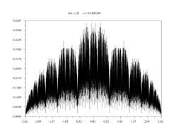
Théorie analytique des nombres
La théorie analytique des nombres est la branche de la théorie des nombres qui utilise les méthodes de l'analyse mathématique. Son premier succès majeur fut l'application de l'analyse par Dirichlet pour la démonstration du Théorème de Dirichlet (existence d'une infinité de nombres premiers dans toute progression arithmétique an+b, lorsque a et b sont des entiers premiers entre eux). Les démonstrations du théorème des nombres premiers basées sur la fonction zêta de Riemann représentent une autre étape. Le développement des ramifications de la discipline, reste similaire à celui de la discipline qui fut à son apogée dans les années 1930. La théorie multiplicative des nombres traite de la distribution des nombres premiers, utilisant les séries de Dirichlet comme fonctions génératrices. Il est supposé que les méthodes s'appliqueront finalement aux fonctions L générales, bien que cette théorie soit encore largement hypothétique. La théorie additive des nombres concerne les problèmes typiques comme la conjecture de Goldbach ou le problème de Waring. Les méthodes ont quelque peu évolué. La méthode du cercle de Hardy et Littlewood avait été conçue comme appliquant aux séries entières près du cercle unité dans le plan complexe ; on y pense désormais en termes de somme exponentielle limitée (c'est-à-dire, sur le cercle unité, mais avec les séries entières tronquées). Les besoins de l'approximation diophantiennesont pour les fonctions auxiliaires qui ne sont pas des fonctions génératrices - leurs coefficients sont construits par l'utilisation d'un principe du casier - et impliquent plusieurs variables complexes. Les champs de l'approximation diophantienne et la théorie transcendantale ont pris de l'expansion, au point que les techniques ont été appliquées à la Conjecture de Mordell. Le plus grand changement technique unique après 1950 fut le développement des méthodes du crible comme un outil auxiliaire, particulièrement dans les problèmes multiplicatifs. Elles sont combinatoires par nature, et plutôt variées. Les utilisations de la théorie probabiliste des nombres sont aussi souvent citées - formes d'assertions de distributions aléatoires sur les nombres premiers, par exemple. Celles-ci n'ont pas reçu une forme définitive. La branche extrême de la théorie combinatoire a en retour été très influencée par la valeur placée dans la théorie analytique des nombres sur des limites quantitatives supérieures et inférieures.Théorie analytique des nombres
21:31 Publié dans Théorie analytique des nombres | Lien permanent | Commentaires (0) | | del.icio.us | | Digg | Facebook
Vladimir Vapnik
Vladimir Vapnik
|
|
Cet article est une ébauche concernant un mathématicien.
Vous pouvez partager vos connaissances en l’améliorant (comment ?) selon les recommandations des projets correspondants.
|
Vladimir Naumovich Vapnik est l'un des principaux contributeurs à la théorie de Vapnik-Chervonenkis. En 1995 il est nommé professeur d'informatique et de statistiques au Royal Holloway College, à l'Université de Londres. Aux laboratoires Bell d'AT&T de 1991 à 2001?, Vladimir Vapnik et ses collègues développent la théorie des machines à support vectoriel (aussi appelées "machines à vecteurs de support", ou encore "séparateurs à vaste marge"), dont ils démontrent l'intérêt dans nombre des problèmatiques importantes de l'apprentissage des machines et des réseaux de neurones, tels que la reconnaissance de caractères. Il travaille désormais aux laboratoires NEC de Princeton, dans le New Jersey, aux États-Unis, ainsi qu'à l'université Columbia, à New York. En 2006, Vladimir Vapnik est admis à l'Académie Nationale d'Ingénierie des Etats-Unis.
Né en Union Soviétique, il obtient en 1958 un mastère de mathématiques à l'Université d'État d'Ouzbékistan, à Samarkand, en Ouzbékistan, puis obtient en 1964 un doctorat destatistiques à l'Institut des Sciences de Contrôle, à Moscou. Il travaille dans ce même institut de 1961 à 1990, et en devient le directeur du département de recherche en informatique.
Sommaire[masquer] |
Bibliographie [modifier]
Liens internes [modifier]
Liens externes [modifier]
Sources [modifier]
21:29 Publié dans Vladimir Vapnik | Lien permanent | Commentaires (0) | | del.icio.us | | Digg | Facebook
Théorème de Rao-Blackwell
Le théorème de Rao-Blackwell permet à partir d'un estimateur (statistique) de construire un estimateur plus précis grâce à l'usage d'une statistique exhaustive. L'avantage de ce théorème est que l'estimateur initial n'a pas nécessairement besoin d'être très bon pour que l'estimateur que ce théorème construit fournisse de bons résultats. Il suffit en effet que l'estimateur de départ soit sans biais pour pouvoir construire un nouvel estimateur. L'estimateur de départ n'a entre autres pas besoin d'être convergent ou efficace.Théorème de Rao-Blackwell
Sommaire[masquer] |
Si δ est un estimateur sans biais et S une statistique exhaustive alors l'estimateur augmenté Dans le cas multiparamétrique où l'estimateur et le paramètre sont en dimensions plus grands que 1 on remplace la variance par la matrice de variance-covariance. Le théorème de Rao-Blackwell donne alors: Quel que soit A défini positif l'erreur quadratique en utilisant le produit scalaire défini par A est toujours plus faible pour l'estimateur augmenté que pour l'estimateur initial. Le fait de pouvoir prendre n'importe quel produit scalaire et non seulement le produit scalaire usuel peut être très utile pour que les différentes composantes ne soit pas normés de la même façon. Ceci peut par exemple être le cas quand si une erreur sur l'une ou l'autre des composantes "coute plus cher" on pourra choisir une matrice de produit scalaire en fonction. L'estimateur augmenté sera toujours préférable même avec ce produit scalaire non usuel. En fait le théorème de Rao Blackwell donne légèrement plus vu qu'il dit que quelle que soit la fonction de perte convexe L On considère donc n variables aléatoires Xi iid distribués selon des lois de Poisson de paramètre λ et l'on cherche à estimer e − λ. On peut montrer assez facilement en considérant lecritère de factorisation que On peut montrer que: δ1 est tout comme δ0 un estimateur de e − λ mais a l'avantage d'être beaucoup plus précis grâce à l'application du théorème de Rao–Blackwell. On peut montrer que En fait bien que Théorème [modifier]
 à une variance plus faible que la variance de l'estimateur initial. L'estimateur augmenté est donc toujours plus précis que l'estimateur initial si on l'augmente d'une statistique exhaustive.
 . L'estimateur augmenté est donc toujours plus précis et ce quelle que soit la définition (raisonnable) que l'on donne à "précis".
Exemple [modifier]
 est une statistique exhaustive. Pour montrer l'intérêt de ce théorème on prend un estimateur grossier de e − λ: δ0 = δ(X1,0) qui vaut 1 si X1 = 0 et 0 sinon. Cet estimateur ne prend en compte qu'une seule valeur de X alors qu'on en dispose de n et il ne donne pour résultat que 0 ou 1 alors que la valeur de e − λ appartient à l'intervalle ]0,1] et ne vaut sans doute pas 1. (si c'était le cas Xi vaudrait 0 de façon déterministe et on s'en serai aperçu en regardant les données). Pourtant bien que cet estimateur soit très grossier l'estimateur augmenté obtenu est très bon et on peut même montrer qu'il est optimal. L'estimateur augmenté vaut:

 est un estimateur optimal de λ (Voir Théorème de Lehman Scheffé) mais que l'estimateur optimal pour e − λ est différent de
  . soit un estimateur convergent de e − λ c'est un estimateur de relativement mauvaise qualité car il est biaisé et qu'en l'estimant de la sorte on fait une erreur systématique sur l'estimation. De façon général il peut être intéressant pour estimer f(λ) de construire un estimateur spécifique plutôt que de calculer la valeur prise par f par l'estimateur de λ.
voir aussi [modifier]
Références [modifier]
Liens externes [modifier]
21:28 Publié dans Théorème de Rao-Blackwell | Lien permanent | Commentaires (0) | | del.icio.us | | Digg | Facebook
Mathematics Genealogy Project
146634 records as of 11 December 2010 20 October 2010—Today we have made an additional feature available to improve the display of mathematics in dissertation titles. We now support standard LaTeX code to be displayed using the MathJax package. Please enclose any LaTeX code in submissions between dollar signs ($) to ensure the smoothest implementation of this. To see an example of a thesis title rendered using MathJax, see the page for James Angelos. 20 October 2010—We recently experienced difficulties with our server that may have resulted in data submissions made between 9 October 2010 and 18 October 2010 not having been received. If you submitted new data or data updates in that period, we encourage you to resubmit them to ensure they are published in a timely manner. Announcements are archived on the news page.
View the growth of the genealogy projectNews
21:26 Publié dans Mathematics Genealogy Project | Lien permanent | Commentaires (0) | | del.icio.us | | Digg | Facebook
Calyampudi Radhakrishna Rao
Calyampudi Radhakrishna Rao
|
|
Cet article est une ébauche concernant un mathématicien.
Vous pouvez partager vos connaissances en l’améliorant (comment ?) selon les recommandations des projets correspondants.
|
Calyampudi Radhakrishna Rao est un célèbre statisticien indien, né en septembre 1920. Il est actuellement professeur émérite à l'Université de Penn. Il est né à Hadagali dans l'État de Karnataka. Il possède une maîtrise en mathématiques de l'Université Andhra, et une maîtrise en statiques de l'Université de Calcutta reçue en 1943. Rao a travaillé à l'Institut indien de statistiques (ISI) et au Museum of Anthropology de Cambridge avant d'obtenir un doctorat au King's College (Cambridge) sous la direction de Ronald Aylmer Fisher en 1948. Parmi ses découvertes les plus célèbres, on lui doit la borne de Cramér-Rao (connue sous le nom de borne FDCR, ou inégalité de Rao-Cramér), et le Théorème de Rao-Blackwell relatant tous deux la qualité des estimateurs. Parmi les autres domaines dans lesquels il a travaillé, on peut citer l'analyse vectorielle et la géométrie différentielle. Rao est lauréat de la médaille Wilks (en) ; membre de huit Académies nationales d'Inde, du Royaume-Uni, des États-Unis et d'Italie, il a reçu une douzaine de prix, médailles, et autres récompenses pour ses contributions en statistiques et en science plus généralement. Rao a été récompensé par la National Medal of Science des États-Unis, la plus haute distinction américaine pour l'ensemble de ses travaux dans le domaine de la recherche scientifique en juin 2002.
Sommaire[masquer] |
(en) M. H. DeGroot A Conversation with C.R. Rao, Statistical Science, 2 (1987), 53-67.Référence [modifier]
Voir aussi [modifier]
Articles connexes [modifier]
Liens externes [modifier]
21:25 Publié dans Calyampudi Radhakrishna Rao, Mathématiciens | Lien permanent | Commentaires (0) | | del.icio.us | | Digg | Facebook
A history of Zero
A history of Zero
| Ancient Indian Mathematics index | History Topics Index |
One of the commonest questions which the readers of this archive ask is: Who discovered zero? Why then have we not written an article on zero as one of the first in the archive? The reason is basically because of the difficulty of answering the question in a satisfactory form. If someone had come up with the concept of zero which everyone then saw as a brilliant innovation to enter mathematics from that time on, the question would have a satisfactory answer even if we did not know which genius invented it. The historical record, however, shows quite a different path towards the concept. Zero makes shadowy appearances only to vanish again almost as if mathematicians were searching for it yet did not recognise its fundamental significance even when they saw it.
The first thing to say about zero is that there are two uses of zero which are both extremely important but are somewhat different. One use is as an empty place indicator in our place-value number system. Hence in a number like 2106 the zero is used so that the positions of the 2 and 1 are correct. Clearly 216 means something quite different. The second use of zero is as a number itself in the form we use it as 0. There are also different aspects of zero within these two uses, namely the concept, the notation, and the name. (Our name "zero" derives ultimately from the Arabic sifr which also gives us the word "cipher".)
Neither of the above uses has an easily described history. It just did not happen that someone invented the ideas, and then everyone started to use them. Also it is fair to say that the number zero is far from an intuitive concept. Mathematical problems started as 'real' problems rather than abstract problems. Numbers in early historical times were thought of much more concretely than the abstract concepts which are our numbers today. There are giant mental leaps from 5 horses to 5 "things" and then to the abstract idea of "five". If ancient peoples solved a problem about how many horses a farmer needed then the problem was not going to have 0 or -23 as an answer.
One might think that once a place-value number system came into existence then the 0 as an empty place indicator is a necessary idea, yet the Babylonians had a place-value number system without this feature for over 1000 years. Moreover there is absolutely no evidence that the Babylonians felt that there was any problem with the ambiguity which existed. Remarkably, original texts survive from the era of Babylonian mathematics. The Babylonians wrote on tablets of unbaked clay, using cuneiform writing. The symbols were pressed into soft clay tablets with the slanted edge of a stylus and so had a wedge-shaped appearance (and hence the name cuneiform). Many tablets from around 1700 BC survive and we can read the original texts. Of course their notation for numbers was quite different from ours (and not based on 10 but on 60) but to translate into our notation they would not distinguish between 2106 and 216 (the context would have to show which was intended). It was not until around 400 BC that the Babylonians put two wedge symbols into the place where we would put zero to indicate which was meant, 216 or 21 '' 6.
The two wedges were not the only notation used, however, and on a tablet found at Kish, an ancient Mesopotamian city located east of Babylon in what is today south-central Iraq, a different notation is used. This tablet, thought to date from around 700 BC, uses three hooks to denote an empty place in the positional notation. Other tablets dated from around the same time use a single hook for an empty place. There is one common feature to this use of different marks to denote an empty position. This is the fact that it never occured at the end of the digits but always between two digits. So although we find 21 '' 6 we never find 216 ''. One has to assume that the older feeling that the context was sufficient to indicate which was intended still applied in these cases.
If this reference to context appears silly then it is worth noting that we still use context to interpret numbers today. If I take a bus to a nearby town and ask what the fare is then I know that the answer "It's three fifty" means three pounds fifty pence. Yet if the same answer is given to the question about the cost of a flight from Edinburgh to New York then I know that three hundred and fifty pounds is what is intended.
We can see from this that the early use of zero to denote an empty place is not really the use of zero as a number at all, merely the use of some type of punctuation mark so that the numbers had the correct interpretation.
Now the ancient Greeks began their contributions to mathematics around the time that zero as an empty place indicator was coming into use in Babylonian mathematics. The Greeks however did not adopt a positional number system. It is worth thinking just how significant this fact is. How could the brilliant mathematical advances of the Greeks not see them adopt a number system with all the advantages that the Babylonian place-value system possessed? The real answer to this question is more subtle than the simple answer that we are about to give, but basically the Greek mathematical achievements were based on geometry. Although Euclid's Elements contains a book on number theory, it is based on geometry. In other words Greek mathematicians did not need to name their numbers since they worked with numbers as lengths of lines. Numbers which required to be named for records were used by merchants, not mathematicians, and hence no clever notation was needed.
Now there were exceptions to what we have just stated. The exceptions were the mathematicians who were involved in recording astronomical data. Here we find the first use of the symbol which we recognise today as the notation for zero, for Greek astronomers began to use the symbol O. There are many theories why this particular notation was used. Some historians favour the explanation that it is omicron, the first letter of the Greek word for nothing namely "ouden". Neugebauer, however, dismisses this explanation since the Greeks already used omicron as a number - it represented 70 (the Greek number system was based on their alphabet). Other explanations offered include the fact that it stands for "obol", a coin of almost no value, and that it arises when counters were used for counting on a sand board. The suggestion here is that when a counter was removed to leave an empty column it left a depression in the sand which looked like O.
Ptolemy in the Almagest written around 130 AD uses the Babylonian sexagesimal system together with the empty place holder O. By this time Ptolemy is using the symbol both between digits and at the end of a number and one might be tempted to believe that at least zero as an empty place holder had firmly arrived. This, however, is far from what happened. Only a few exceptional astronomers used the notation and it would fall out of use several more times before finally establishing itself. The idea of the zero place (certainly not thought of as a number by Ptolemy who still considered it as a sort of punctuation mark) makes its next appearance in Indian mathematics.
The scene now moves to India where it is fair to say the numerals and number system was born which have evolved into the highly sophisticated ones we use today. Of course that is not to say that the Indian system did not owe something to earlier systems and many historians of mathematics believe that the Indian use of zero evolved from its use by Greek astronomers. As well as some historians who seem to want to play down the contribution of the Indians in a most unreasonable way, there are also those who make claims about the Indian invention of zero which seem to go far too far. For example Mukherjee in [6] claims:-
... the mathematical conception of zero ... was also present in the spiritual form from 17 000 years back in India.
What is certain is that by around 650AD the use of zero as a number came into Indian mathematics. The Indians also used a place-value system and zero was used to denote an empty place. In fact there is evidence of an empty place holder in positional numbers from as early as 200AD in India but some historians dismiss these as later forgeries. Let us examine this latter use first since it continues the development described above.
In around 500AD Aryabhata devised a number system which has no zero yet was a positional system. He used the word "kha" for position and it would be used later as the name for zero. There is evidence that a dot had been used in earlier Indian manuscripts to denote an empty place in positional notation. It is interesting that the same documents sometimes also used a dot to denote an unknown where we might use x. Later Indian mathematicians had names for zero in positional numbers yet had no symbol for it. The first record of the Indian use of zero which is dated and agreed by all to be genuine was written in 876.
We have an inscription on a stone tablet which contains a date which translates to 876. The inscription concerns the town of Gwalior, 400 km south of Delhi, where they planted a garden 187 by 270 hastas which would produce enough flowers to allow 50 garlands per day to be given to the local temple. Both of the numbers 270 and 50 are denoted almost as they appear today although the 0 is smaller and slightly raised.
We now come to considering the first appearance of zero as a number. Let us first note that it is not in any sense a natural candidate for a number. From early times numbers are words which refer to collections of objects. Certainly the idea of number became more and more abstract and this abstraction then makes possible the consideration of zero and negative numbers which do not arise as properties of collections of objects. Of course the problem which arises when one tries to consider zero and negatives as numbers is how they interact in regard to the operations of arithmetic, addition, subtraction, multiplication and division. In three important books the Indian mathematicians Brahmagupta, Mahavira and Bhaskara tried to answer these questions.
Brahmagupta attempted to give the rules for arithmetic involving zero and negative numbers in the seventh century. He explained that given a number then if you subtract it from itself you obtain zero. He gave the following rules for addition which involve zero:-
The sum of zero and a negative number is negative, the sum of a positive number and zero is positive, the sum of zero and zero is zero.
Subtraction is a little harder:-
A negative number subtracted from zero is positive, a positive number subtracted from zero is negative, zero subtracted from a negative number is negative, zero subtracted from a positive number is positive, zero subtracted from zero is zero.
Brahmagupta then says that any number when multiplied by zero is zero but struggles when it comes to division:-
A positive or negative number when divided by zero is a fraction with the zero as denominator. Zero divided by a negative or positive number is either zero or is expressed as a fraction with zero as numerator and the finite quantity as denominator. Zero divided by zero is zero.
Really Brahmagupta is saying very little when he suggests that n divided by zero is n/0. Clearly he is struggling here. He is certainly wrong when he then claims that zero divided by zero is zero. However it is a brilliant attempt from the first person that we know who tried to extend arithmetic to negative numbers and zero.
In 830, around 200 years after Brahmagupta wrote his masterpiece, Mahavira wrote Ganita Sara Samgraha which was designed as an updating of Brahmagupta's book. He correctly states that:-
... a number multiplied by zero is zero, and a number remains the same when zero is subtracted from it.
However his attempts to improve on Brahmagupta's statements on dividing by zero seem to lead him into error. He writes:-
A number remains unchanged when divided by zero.
Since this is clearly incorrect my use of the words "seem to lead him into error" might be seen as confusing. The reason for this phrase is that some commentators on Mahavira have tried to find excuses for his incorrect statement.
Bhaskara wrote over 500 years after Brahmagupta. Despite the passage of time he is still struggling to explain division by zero. He writes:-
A quantity divided by zero becomes a fraction the denominator of which is zero. This fraction is termed an infinite quantity. In this quantity consisting of that which has zero for its divisor, there is no alteration, though many may be inserted or extracted; as no change takes place in the infinite and immutable God when worlds are created or destroyed, though numerous orders of beings are absorbed or put forth.
So Bhaskara tried to solve the problem by writing n/0 = ∞. At first sight we might be tempted to believe that Bhaskara has it correct, but of course he does not. If this were true then 0 times ∞ must be equal to every number n, so all numbers are equal. The Indian mathematicians could not bring themselves to the point of admitting that one could not divide by zero. Bhaskara did correctly state other properties of zero, however, such as 02 = 0, and √0 = 0.
Perhaps we should note at this point that there was another civilisation which developed a place-value number system with a zero. This was the Maya people who lived in central America, occupying the area which today is southern Mexico, Guatemala, and northern Belize. This was an old civilisation but flourished particularly between 250 and 900. We know that by 665 they used a place-value number system to base 20 with a symbol for zero. However their use of zero goes back further than this and was in use before they introduced the place-valued number system. This is a remarkable achievement but sadly did not influence other peoples.
You can see a separate article about Mayan mathematics.
The brilliant work of the Indian mathematicians was transmitted to the Islamic and Arabic mathematicians further west. It came at an early stage for al-Khwarizmi wrote Al'Khwarizmi on the Hindu Art of Reckoning which describes the Indian place-value system of numerals based on 1, 2, 3, 4, 5, 6, 7, 8, 9, and 0. This work was the first in what is now Iraq to use zero as a place holder in positional base notation. Ibn Ezra, in the 12th century, wrote three treatises on numbers which helped to bring the Indian symbols and ideas of decimal fractions to the attention of some of the learned people in Europe. The Book of the Number describes the decimal system for integers with place values from left to right. In this work ibn Ezra uses zero which he calls galgal (meaning wheel or circle). Slightly later in the 12thcentury al-Samawal was writing:-
If we subtract a positive number from zero the same negative number remains. ... if we subtract a negative number from zero the same positive number remains.
The Indian ideas spread east to China as well as west to the Islamic countries. In 1247 the Chinese mathematician Ch'in Chiu-Shao wrote Mathematical treatise in nine sections which uses the symbol O for zero. A little later, in 1303, Zhu Shijie wrote Jade mirror of the four elements which again uses the symbol O for zero.
Fibonacci was one of the main people to bring these new ideas about the number system to Europe. As the authors of [12] write:-
An important link between the Hindu-Arabic number system and the European mathematics is the Italian mathematician Fibonacci.
In Liber Abaci he described the nine Indian symbols together with the sign 0 for Europeans in around 1200 but it was not widely used for a long time after that. It is significant that Fibonacci is not bold enough to treat 0 in the same way as the other numbers 1, 2, 3, 4, 5, 6, 7, 8, 9 since he speaks of the "sign" zero while the other symbols he speaks of as numbers. Although clearly bringing the Indian numerals to Europe was of major importance we can see that in his treatment of zero he did not reach the sophistication of the Indians Brahmagupta, Mahavira and Bhaskara nor of the Arabic and Islamic mathematicians such as al-Samawal.
One might have thought that the progress of the number systems in general, and zero in particular, would have been steady from this time on. However, this was far from the case. Cardan solved cubic and quartic equations without using zero. He would have found his work in the 1500's so much easier if he had had a zero but it was not part of his mathematics. By the 1600's zero began to come into widespread use but still only after encountering a lot of resistance.
Of course there are still signs of the problems caused by zero. Recently many people throughout the world celebrated the new millennium on 1 January 2000. Of course they celebrated the passing of only 1999 years since when the calendar was set up no year zero was specified. Although one might forgive the original error, it is a little surprising that most people seemed unable to understand why the third millennium and the 21st century begin on 1 January 2001. Zero is still causing problems!
References (14 books/articles)
Other Web sites:
Astroseti (A Spanish translation of this article)
Article by: J J O'Connor and E F Robertson
JOC/EFR November 2000
The URL of this page is:
http://www-history.mcs.st-andrews.ac.uk/HistTopics/Zero.html
Source : http://www-groups.dcs.st-and.ac.uk/~history/HistTopics/Ze...
12:03 Publié dans A history of Zero | Lien permanent | Commentaires (0) | | del.icio.us | | Digg | Facebook
Pythagoras's theorem in Babylonian mathematics
Pythagoras's theorem in Babylonian mathematics
| Babylonian index | History Topics Index |
Pythagoras's theorem in Babylonian mathematics
In this article we examine four Babylonian tablets which all have some connection with Pythagoras's theorem. Certainly the Babylonians were familiar with Pythagoras's theorem. A translation of a Babylonian tablet which is preserved in the British museum goes as follows:-
4 is the length and 5 the diagonal. What is the breadth ?
Its size is not known.
4 times 4 is 16.
5 times 5 is 25.
You take 16 from 25 and there remains 9.
What times what shall I take in order to get 9 ?
3 times 3 is 9.
3 is the breadth.
All the tablets we wish to consider in detail come from roughly the same period, namely that of the Old Babylonian Empire which flourished in Mesopotamia between 1900 BC and 1600 BC.
Here is a map of the region where the Babylonian civilisation flourished.
The article Babylonian mathematics gives some background to how the civilisation came about and the mathematical background which they inherited.
The four tablets which interest us here we will call the Yale tablet YBC 7289, Plimpton 322 (shown below), the Susa tablet, and the Tell Dhibayi tablet. Let us say a little about these tablets before describing the mathematics which they contain.
The Yale tablet YBC 7289 which we describe is one of a large collection of tablets held in the Yale Babylonian collection of Yale University. It consists of a tablet on which a diagram appears. The diagram is a square of side 30 with the diagonals drawn in. The tablet and its significance was first discussed in [5] and recently in [18].
Plimpton 322 is the tablet numbered 322 in the collection of G A Plimpton housed in Columbia University.
You can see from the picture that the top left hand corner of the tablet is damaged as and there is a large chip out of the tablet around the middle of the right hand side. Its date is not known accurately but it is put at between 1800 BC and 1650 BC. It is thought to be only part of a larger tablet, the remainder of which has been destroyed, and at first it was thought, as many such tablets are, to be a record of commercial transactions. However in [5] Neugebauer and Sachs gave a new interpretation and since then it has been the subject of a huge amount of interest.
The Susa tablet was discovered at the present town of Shush in the Khuzistan region of Iran. The town is about 350 km from the ancient city of Babylon. W K Loftus identified this as an important archaeological site as early as 1850 but excavations were not carried out until much later. The particular tablet which interests us here investigates how to calculate the radius of a circle through the vertices of an isosceles triangle.
Finally the Tell Dhibayi tablet was one of about 500 tablets found near Baghdad by archaeologists in 1962. Most relate to the administration of an ancient city which flourished in the time of Ibalpiel II of Eshunna and date from around 1750. The particular tablet which concerns us is not one relating to administration but one which presents a geometrical problem which asks for the dimensions of a rectangle whose area and diagonal are known.
Before looking at the mathematics contained in these four tablets we should say a little about their significance in understanding the scope of Babylonian mathematics. Firstly we should be careful not to read into early mathematics ideas which we can see clearly today yet which were never in the mind of the author. Conversely we must be careful not to underestimate the significance of the mathematics just because it has been produced by mathematicians who thought very differently from today's mathematicians. As a final comment on what these four tablets tell us of Babylonian mathematics we must be careful to realise that almost all of the mathematical achievements of the Babylonians, even if they were all recorded on clay tablets, will have been lost and even if these four may be seen as especially important among those surviving they may not represent the best of Babylonian mathematics.
There is no problem understanding what the Yale tablet YBC 7289 is about. 
Here is a Diagram of Yale tablet
It has on it a diagram of a square with 30 on one side, the diagonals are drawn in and near the centre is written 1,24,51,10 and 42,25,35. Of course these numbers are written in Babylonian numerals to base 60. See our article on Babylonian numerals. Now the Babylonian numbers are always ambiguous and no indication occurs as to where the integer part ends and the fractional part begins. Assuming that the first number is 1; 24,51,10 then converting this to a decimal gives 1.414212963 while √2 = 1.414213562. Calculating 30  [ 1;24,51,10 ] gives 42;25,35 which is the second number. The diagonal of a square of side 30 is found by multiplying 30 by the approximation to √2.
This shows a nice understanding of Pythagoras's theorem. However, even more significant is the question how the Babylonians found this remarkably good approximation to √2. Several authors, for example see [2] and [4], conjecture that the Babylonians used a method equivalent to Heron's method. The suggestion is that they started with a guess, say x. They then found e = x2 - 2 which is the error. Then
(x - e/2x)2 = x2 - e + (e/2x)2 = 2 + (e/2x)2
and they had a better approximation since if e is small then (e/2x)2 will be very small. Continuing the process with this better approximation to √2 yieds a still better approximation and so on. In fact as Joseph points out in [4], one needs only two steps of the algorithm if one starts with x = 1 to obtain the approximation 1;24,51,10.
This is certainly possible and the Babylonians' understanding of quadratics adds some weight to the claim. However there is no evidence of the algorithm being used in any other cases and its use here must remain no more than a fairly remote possibility. May I [EFR] suggest an alternative. The Babylonians produced tables of squares, in fact their whole understanding of multiplication was built round squares, so perhaps a more obvious approach for them would have been to make two guesses, one high and one low say a and b. Take their average (a + b)/2 and square it. If the square is greater than 2 then replace bby this better bound, while if the square is less than 2 then replace a by (a + b)/2. Continue with the algorithm.
Now this certainly takes many more steps to reach the sexagesimal approximation 1;24,51,10. In fact starting with a = 1 and b = 2 it takes 19 steps as the table below shows:
step decimal sexagesimal1 1.500000000 1;29,59,59
2 1.250000000 1;14,59,59
3 1.375000000 1;22,29,59
4 1.437500000 1;26,14,59
5 1.406250000 1;24,22,29
6 1.421875000 1;25,18,44
7 1.414062500 1;24,50,37
8 1.417968750 1;25, 4,41
9 1.416015625 1;24,57,39
10 1.415039063 1;24,54, 8
11 1.414550781 1;24,52,22
12 1.414306641 1;24,51;30
13 1.414184570 1;24,51; 3
14 1.414245605 1;24,51;17
15 1.414215088 1;24,51;10
16 1.414199829 1;24,51; 7
17 1.414207458 1;24,51; 8
18 1.414211273 1;24,51; 9
19 1.414213181 1;24,51;10
However, the Babylonians were not frightened of computing and they may have been prepared to continue this straightforward calculation until the answer was correct to the third sexagesimal place.
Next we look again at Plimpton 322
The tablet has four columns with 15 rows. The last column is the simplest to understand for it gives the row number and so contains 1, 2, 3, ... , 15. The remarkable fact which Neugebauer and Sachs pointed out in [5] is that in every row the square of the number c in column 3 minus the square of the number b in column 2 is a perfect square, say h.
c2 - b2 = h2
So the table is a list of Pythagorean integer triples. Now this is not quite true since Neugebauer and Sachs believe that the scribe made four transcription errors, two in each column and this interpretation is required to make the rule work. The errors are readily seen to be genuine errors, however, for example 8,1 has been copied by the scribe as 9,1.
The first column is harder to understand, particularly since damage to the tablet means that part of it is missing. However, using the above notation, it is seen that the first column is just (c/h)2. Now so far so good, but if one were writing down Pythagorean triples one would find much easier ones than those which appear in the table. For example the Pythagorean triple 3, 4 , 5 does not appear neither does 5, 12, 13 and in fact the smallest Pythagorean triple which does appear is 45, 60, 75 (15 times 3, 4 , 5). Also the rows do not appear in any logical order except that the numbers in column 1 decrease regularly. The puzzle then is how the numbers were found and why are these particular Pythagorean triples are given in the table.
Several historians (see for example [2]) have suggested that column 1 is connected with the secant function. However, as Joseph comments [4]:-
This interpretation is a trifle fanciful.
Zeeman has made a fascinating observation. He has pointed out that if the Babylonians used the formulas h = 2mn, b = m2-n2, c = m2+n2 to generate Pythagorean triples then there are exactly 16 triples satisfying n ≤ 60, 30° ≤ t ≤ 45°, and tan2t = h2/b2 having a finite sexagesimal expansion (which is equivalent to m, n, b having 2, 3, and 5 as their only prime divisors). Now 15 of the 16 Pythagorean triples satisfying Zeeman's conditions appear in Plimpton 322. Is it the earliest known mathematical classification theorem? Although I cannot believe that Zeeman has it quite right, I do feel that his explanation must be on the right track.
To give a fair discussion of Plimpton 322 we should add that not all historians agree that this tablet concerns Pythagorean triples. For example Exarchakos, in [17], claims that the tablet is connected with the solution of quadratic equations and has nothing to do with Pythagorean triples:-
... we prove that in this tablet there is no evidence whatsoever that the Babylonians knew the Pythagorean theorem and the Pythagorean triads.
I feel that the arguments are weak, particularly since there are numerous tablets which show that the Babylonians of this period had a good understanding of Pythagoras's theorem. Other authors, although accepting that Plimpton 322 is a collection of Pythagorean triples, have argued that they had, as Viola writes in [31], a practical use in giving a:-
... general method for the approximate computation of areas of triangles.
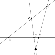
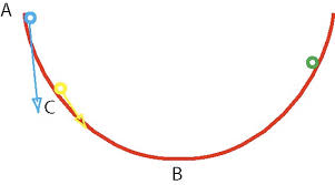
The Susa tablet sets out a problem about an isosceles triangle with sides 50, 50 and 60. The problem is to find the radius of the circle through the three vertices.
Here is a Diagram of Susa tablet
Here we have labelled the triangle A, B, C and the centre of the circle is O. The perpendicular AD is drawn from A to meet the side BC. Now the triangle ABD is a right angled triangle so, using Pythagoras's theorem AD2 = AB2 - BD2, so AD = 40. Let the radius of the circle by x. Then AO = OB = x and OD = 40 - x. Using Pythagoras's theorem again on the triangle OBD we have
x2 = OD2 + DB2.
So
x2 = (40-x)2 + 302
giving x2 = 402 - 80x + x2 + 302
and so 80x = 2500 or, in sexagesimal, x = 31;15.
Finally consider the problem from the Tell Dhibayi tablet. It asks for the sides of a rectangle whose area is 0;45 and whose diagonal is 1;15. Now this to us is quite an easy exercise in solving equations. If the sides are x, y we have xy = 0.75 and x2 + y2 = (1.25)2. We would substitute y = 0.75/x into the second equation to obtain a quadratic in x2 which is easily solved. This however is not the method of solution given by the Babylonians and really that is not surprising since it rests heavily on our algebraic understanding of equations. The way the Tell Dhibayi tablet solves the problem is, I would suggest, actually much more interesting than the modern method.
Here is the method from the Tell Dhibayi tablet. We preserve the modern notation x and y as each step for clarity but we do the calculations in sexagesimal notation (as of course does the tablet).
Compute 2xy = 1;30.
Subtract from x2 + y2 = 1;33,45 to get x2 + y2 - 2xy = 0;3,45.
Take the square root to obtain x - y = 0;15.
Divide by 2 to get (x - y)/2 = 0;7,30.
Divide x2 + y2 - 2xy = 0;3,45 by 4 to get x2/4 + y2/4 - xy/2 = 0;0,56,15.
Add xy = 0;45 to get x2/4 + y2/4 + xy/2 = 0;45,56,15.
Take the square root to obtain (x + y)/2 = 0;52,30.
Add (x + y)/2 = 0;52,30 to (x - y)/2 = 0;7,30 to get x = 1.
Subtract (x - y)/2 = 0;7,30 from (x + y)/2 = 0;52,30 to get y = 0;45.
Hence the rectangle has sides x = 1 and y = 0;45.
Is this not a beautiful piece of mathematics! Remember that it is 3750 years old. We should be grateful to the Babylonians for recording this little masterpiece on tablets of clay for us to appreciate today.
References (31 books/articles)
Other Web sites:
Astroseti (A Spanish translation of this article)
Article by: J J O'Connor and E F Robertson
JOC/EFR December 2000
The URL of this page is:
http://www-history.mcs.st-andrews.ac.uk/HistTopics/Babylonian_Pythagoras.html
Source : http://www-groups.dcs.st-and.ac.uk/~history/HistTopics/Ba...
12:02 Publié dans Pythagoras's theorem in Babylonian mathematics | Lien permanent | Commentaires (0) | | del.icio.us | | Digg | Facebook
Babylonian numerals
Babylonian numerals
| Babylonian index | History Topics Index |
The Babylonian civilisation in Mesopotamia replaced the Sumerian civilisation and the Akkadian civilisation. We give a little historical background to these events in our article Babylonian mathematics. Certainly in terms of their number system the Babylonians inherited ideas from the Sumerians and from the Akkadians. From the number systems of these earlier peoples came the base of 60, that is the sexagesimal system. Yet neither the Sumerian nor the Akkadian system was a positional system and this advance by the Babylonians was undoubtedly their greatest achievement in terms of developing the number system. Some would argue that it was their biggest achievement in mathematics.
Often when told that the Babylonian number system was base 60 people's first reaction is: what a lot of special number symbols they must have had to learn. Now of course this comment is based on knowledge of our own decimal system which is a positional system with nine special symbols and a zero symbol to denote an empty place. However, rather than have to learn 10 symbols as we do to use our decimal numbers, the Babylonians only had to learn two symbols to produce their base 60 positional system.
Now although the Babylonian system was a positional base 60 system, it had some vestiges of a base 10 system within it. This is because the 59 numbers, which go into one of the places of the system, were built from a 'unit' symbol and a 'ten' symbol.

Here are the 59 symbols built from these two symbols
Now given a positional system one needs a convention concerning which end of the number represents the units. For example the decimal 12345 represents
1
If one thinks about it this is perhaps illogical for we read from left to right so when we read the first digit we do not know its value until we have read the complete number to find out how many powers of 10 are associated with this first place. The Babylonian sexagesimal positional system places numbers with the same convention, so the right most position is for the units up to 59, the position one to the left is for 60 n where 1 ≤ n ≤ 59, etc. Now we adopt a notation where we separate the numerals by commas so, for example, 1,57,46,40 represents the sexagesimal number
1
which, in decimal notation is 424000.

Here is 1,57,46,40 in Babylonian numerals
Now there is a potential problem with the system. Since two is represented by two characters each representing one unit, and 61 is represented by the one character for a unit in the first place and a second identical character for a unit in the second place then the Babylonian sexagesimal numbers 1,1 and 2 have essentially the same representation. However, this was not really a problem since the spacing of the characters allowed one to tell the difference. In the symbol for 2 the two characters representing the unit touch each other and become a single symbol. In the number 1,1 there is a space between them.
A much more serious problem was the fact that there was no zero to put into an empty position. The numbers sexagesimal numbers 1 and 1,0, namely 1 and 60 in decimals, had exactly the same representation and now there was no way that spacing could help. The context made it clear, and in fact despite this appearing very unsatisfactory, it could not have been found so by the Babylonians. How do we know this? Well if they had really found that the system presented them with real ambiguities they would have solved the problem - there is little doubt that they had the skills to come up with a solution had the system been unworkable. Perhaps we should mention here that later Babylonian civilisations did invent a symbol to indicate an empty place so the lack of a zero could not have been totally satisfactory to them.
An empty place in the middle of a number likewise gave them problems. Although not a very serious comment, perhaps it is worth remarking that if we assume that all our decimal digits are equally likely in a number then there is a one in ten chance of an empty place while for the Babylonians with their sexagesimal system there was a one in sixty chance. Returning to empty places in the middle of numbers we can look at actual examples where this happens.
Here is an example from a cuneiform tablet (actually AO 17264 in the Louvre collection in Paris) in which the calculation to square 147 is carried out. In sexagesimal 147 = 2,27 and squaring gives the number 21609 = 6,0,9.

Here is the Babylonian example of 2,27 squared
Perhaps the scribe left a little more space than usual between the 6 and the 9 than he would have done had he been representing 6,9.
Now if the empty space caused a problem with integers then there was an even bigger problem with Babylonian sexagesimal fractions. The Babylonians used a system of sexagesimal fractions similar to our decimal fractions. For example if we write 0.125 then this is 1/10 + 2/100 + 5/1000 = 1/8. Of course a fraction of the form a/b, in its lowest form, can be represented as a finite decimal fraction if and only if b has no prime divisors other than 2 or 5. So 1/3 has no finite decimal fraction. Similarly the Babylonian sexagesimal fraction 0;7,30 represented 7/60 + 30/3600 which again written in our notation is 1/8.
Since 60 is divisible by the primes 2, 3 and 5 then a number of the form a/b, in its lowest form, can be represented as a finite decimal fraction if and only if b has no prime divisors other than 2, 3 or 5. More fractions can therefore be represented as finite sexagesimal fractions than can as finite decimal fractions. Some historians think that this observation has a direct bearing on why the Babylonians developed the sexagesimal system, rather than the decimal system, but this seems a little unlikely. If this were the case why not have 30 as a base? We discuss this problem in some detail below.
Now we have already suggested the notation that we will use to denote a sexagesimal number with fractional part. To illustrate 10,12,5;1,52,30 represents the number
10
which in our notation is 36725 1/32. This is fine but we have introduced the notation of the semicolon to show where the integer part ends and the fractional part begins. It is the "sexagesimal point" and plays an analogous role to a decimal point. However, the Babylonians has no notation to indicate where the integer part ended and the fractional part began. Hence there was a great deal of ambiguity introduced and "the context makes it clear" philosophy now seems pretty stretched. If I write 10,12,5,1,52,30 without having a notation for the "sexagesimal point" then it could mean any of:
0;10,12, 5, 1,52,30

  10;12, 5, 1,52,30

  10,12; 5, 1,52,30

  10,12, 5; 1,52,30

  10,12, 5, 1;52,30

  10,12, 5, 1,52;30

  10,12, 5, 1,52,30
in addition, of course, to 10, 12, 5, 1, 52, 30, 0 or 0 ; 0, 10, 12, 5, 1, 52, 30 etc.
Finally we should look at the question of why the Babylonians had a number system with a base of 60. The easy answer is that they inherited the base of 60 from the Sumerians but that is no answer at all. It only leads us to ask why the Sumerians used base 60. The first comment would be that we do not have to go back further for we can be fairly certain that the sexagesimal system originated with the Sumerians. The second point to make is that modern mathematicians were not the first to ask such questions. Theon of Alexandria tried to answer this question in the fourth century AD and many historians of mathematics have offered an opinion since then without any coming up with a really convincing answer.
Theon's answer was that 60 was the smallest number divisible by 1, 2, 3, 4, and 5 so the number of divisors was maximised. Although this is true it appears too scholarly a reason. A base of 12 would seem a more likely candidate if this were the reason, yet no major civilisation seems to have come up with that base. On the other hand many measures do involve 12, for example it occurs frequently in weights, money and length subdivisions. For example in old British measures there were twelve inches in a foot, twelve pennies in a shilling etc.
Neugebauer proposed a theory based on the weights and measures that the Sumerians used. His idea basically is that a decimal counting system was modified to base 60 to allow for dividing weights and measures into thirds. Certainly we know that the system of weights and measures of the Sumerians do use 1/3 and 2/3 as basic fractions. However although Neugebauer may be correct, the counter argument would be that the system of weights and measures was a consequence of the number system rather than visa versa.
Several theories have been based on astronomical events. The suggestion that 60 is the product of the number of months in the year (moons per year) with the number of planets (Mercury, Venus, Mars, Jupiter, Saturn) again seems far fetched as a reason for base 60. That the year was thought to have 360 days was suggested as a reason for the number base of 60 by the historian of mathematics Moritz Cantor. Again the idea is not that convincing since the Sumerians certainly knew that the year was longer than 360 days. Another hypothesis concerns the fact that the sun moves through its diameter 720 times during a day and, with 12 Sumerian hours in a day, one can come up with 60.
Some theories are based on geometry. For example one theory is that an equilateral triangle was considered the fundamental geometrical building block by the Sumerians. Now an angle of an equilateral triangle is 60° so if this were divided into 10, an angle of 6° would become the basic angular unit. Now there are sixty of these basic units in a circle so again we have the proposed reason for choosing 60 as a base. Notice this argument almost contradicts itself since it assumes 10 as the basic unit for division!
I [EFR] feel that all of these reasons are really not worth considering seriously. Perhaps I've set up my own argument a little, but the phrase "choosing 60 as a base" which I just used is highly significant. I just do not believe that anyone ever chose a number base for any civilisation. Can you imagine the Sumerians setting set up a committee to decide on their number base - no things just did not happen in that way. The reason has to involve the way that counting arose in the Sumerian civilisation, just as 10 became a base in other civilisations who began counting on their fingers, and twenty became a base for those who counted on both their fingers and toes.
Here is one way that it could have happened. One can count up to 60 using your two hands. On your left hand there are three parts on each of four fingers (excluding the thumb). The parts are divided from each other by the joints in the fingers. Now one can count up to 60 by pointing at one of the twelve parts of the fingers of the left hand with one of the five fingers of the right hand. This gives a way of finger counting up to 60 rather than to 10. Anyone convinced?
A variant of this proposal has been made by others. Perhaps the most widely accepted theory proposes that the Sumerian civilisation must have come about through the joining of two peoples, one of whom had base 12 for their counting and the other having base 5. Although 5 is nothing like as common as 10 as a number base among ancient peoples, it is not uncommon and is clearly used by people who counted on the fingers of one hand and then started again. This theory then supposes that as the two peoples mixed and the two systems of counting were used by different members of the society trading with each other then base 60 would arise naturally as the system everyone understood.
I have heard the same theory proposed but with the two peoples who mixed to produce the Sumerians having 10 and 6 as their number bases. This version has the advantage that there is a natural unit for 10 in the Babylonian system which one could argue was a remnant of the earlier decimal system. One of the nicest things about these theories is that it may be possible to find written evidence of the two mixing systems and thereby give what would essentially amount to a proof of the conjecture. Do not think of history as a dead subject. On the contrary our views are constantly changing as the latest research brings new evidence and new interpretations to light.
References (9 books/articles)
Other Web sites:
Astroseti (A Spanish translation of this article)
Article by: J J O'Connor and E F Robertson
JOC/EFR December 2000
The URL of this page is:
http://www-history.mcs.st-andrews.ac.uk/HistTopics/Babylonian_numerals.html
Source : http://www-groups.dcs.st-and.ac.uk/~history/HistTopics/Ba...
12:01 Publié dans Babylonian numerals | Lien permanent | Commentaires (0) | | del.icio.us | | Digg | Facebook
An overview of Babylonian mathematics
An overview of Babylonian mathematics
| Babylonian index | History Topics Index |
The Babylonians lived in Mesopotamia, a fertile plain between the Tigris and Euphrates rivers.
Here is a map of the region where the civilisation flourished.
The region had been the centre of the Sumerian civilisation which flourished before 3500 BC. This was an advanced civilisation building cities and supporting the people with irrigation systems, a legal system, administration, and even a postal service. Writing developed and counting was based on a sexagesimal system, that is to say base 60. Around 2300 BC the Akkadians invaded the area and for some time the more backward culture of the Akkadians mixed with the more advanced culture of the Sumerians. The Akkadians invented the abacus as a tool for counting and they developed somewhat clumsy methods of arithmetic with addition, subtraction, multiplication and division all playing a part. The Sumerians, however, revolted against Akkadian rule and by 2100 BC they were back in control.
However the Babylonian civilisation, whose mathematics is the subject of this article, replaced that of the Sumerians from around 2000 BC The Babylonians were a Semitic people who invaded Mesopotamia defeating the Sumerians and by about 1900 BC establishing their capital at Babylon.
The Sumerians had developed an abstract form of writing based on cuneiform (i.e. wedge-shaped) symbols. Their symbols were written on wet clay tablets which were baked in the hot sun and many thousands of these tablets have survived to this day. It was the use of a stylus on a clay medium that led to the use of cuneiform symbols since curved lines could not be drawn. The later Babylonians adopted the same style of cuneiform writing on clay tablets.

Here is one of their tablets
Many of the tablets concern topics which, although not containing deep mathematics, nevertheless are fascinating. For example we mentioned above the irrigation systems of the early civilisations in Mesopotamia. These are discussed in [40] where Muroi writes:-
It was an important task for the rulers of Mesopotamia to dig canals and to maintain them, because canals were not only necessary for irrigation but also useful for the transport of goods and armies. The rulers or high government officials must have ordered Babylonian mathematicians to calculate the number of workers and days necessary for the building of a canal, and to calculate the total expenses of wages of the workers.
There are several Old Babylonian mathematical texts in which various quantities concerning the digging of a canal are asked for. They are YBC 4666, 7164, and VAT 7528, all of which are written in Sumerian ..., and YBC 9874 and BM 85196, No. 15, which are written in Akkadian ... . From the mathematical point of view these problems are comparatively simple ...
The Babylonians had an advanced number system, in some ways more advanced than our present systems. It was a positional system with a base of 60 rather than the system with base 10 in widespread use today. For more details of the Babylonian numerals, and also a discussion as to the theories why they used base 60, see our article on Babylonian numerals.
The Babylonians divided the day into 24 hours, each hour into 60 minutes, each minute into 60 seconds. This form of counting has survived for 4000 years. To write 5h 25' 30", i.e. 5 hours, 25 minutes, 30 seconds, is just to write the sexagesimal fraction, 5 25/60 30/3600. We adopt the notation 5; 25, 30 for this sexagesimal number, for more details regarding this notation see our article on Babylonian numerals. As a base 10 fraction the sexagesimal number 5; 25, 30 is 5 4/10 2/100 5/1000 which is written as 5.425 in decimal notation.
Perhaps the most amazing aspect of the Babylonian's calculating skills was their construction of tables to aid calculation. Two tablets found at Senkerah on the Euphrates in 1854 date from 2000 BC. They give squares of the numbers up to 59 and cubes of the numbers up to 32. The table gives 82 = 1,4 which stands for
82 = 1, 4 = 1
and so on up to 592 = 58, 1 (= 58 60 +1 = 3481).
The Babylonians used the formula
ab = [(a + b)2 - a2 - b2]/2
to make multiplication easier. Even better is their formula
ab = [(a + b)2 - (a - b)2]/4
which shows that a table of squares is all that is necessary to multiply numbers, simply taking the difference of the two squares that were looked up in the table then taking a quarter of the answer.
Division is a harder process. The Babylonians did not have an algorithm for long division. Instead they based their method on the fact that
a/b = a
so all that was necessary was a table of reciprocals. We still have their reciprocal tables going up to the reciprocals of numbers up to several billion. Of course these tables are written in their numerals, but using the sexagesimal notation we introduced above, the beginning of one of their tables would look like:
         2          0; 30

         3          0; 20

         4          0; 15

         5          0; 12

         6          0; 10

         8          0; 7, 30

         9          0; 6, 40

        10          0; 6

        12          0; 5

        15          0; 4

        16          0; 3, 45

        18          0; 3, 20

        20          0; 3

        24          0; 2, 30

        25          0; 2, 24

        27          0; 2, 13, 20
Now the table had gaps in it since 1/7, 1/11, 1/13, etc. are not finite base 60 fractions. This did not mean that the Babylonians could not compute 1/13, say. They would write
1/13 = 7/91 = 7
and these values, for example 1/90, were given in their tables. In fact there are fascinating glimpses of the Babylonians coming to terms with the fact that division by 7 would lead to an infinite sexagesimal fraction. A scribe would give a number close to 1/7 and then write statements such as (see for example [5]):-
... an approximation is given since 7 does not divide.
Babylonian mathematics went far beyond arithmetical calculations. In our article on Pythagoras's theorem in Babylonian mathematics we examine some of their geometrical ideas and also some basic ideas in number theory. In this article we now examine some algebra which the Babylonians developed, particularly problems which led to equations and their solution.
We noted above that the Babylonians were famed as constructors of tables. Now these could be used to solve equations. For example they constructed tables for n3 + n2 then, with the aid of these tables, certain cubic equations could be solved. For example, consider the equation
ax3 + bx2 = c.
Let us stress at once that we are using modern notation and nothing like a symbolic representation existed in Babylonian times. Nevertheless the Babylonians could handle numerical examples of such equations by using rules which indicate that they did have the concept of a typical problem of a given type and a typical method to solve it. For example in the above case they would (in our notation) multiply the equation by a2 and divide it by b3 to get
(ax/b)3 + (ax/b)2 = ca2/b3.
Putting y = ax/b this gives the equation
y3 + y2 = ca2/b3
which could now be solved by looking up the n3 + n2 table for the value of n satisfying n3 + n2 = ca2/b3. When a solution was found for y then x was found by x = by/a. We stress again that all this was done without algebraic notation and showed a remarkable depth of understanding.
Again a table would have been looked up to solve the linear equation ax = b. They would consult the 1/n table to find 1/a and then multiply the sexagesimal number given in the table by b. An example of a problem of this type is the following.
Suppose, writes a scribe, 2/3 of 2/3 of a certain quantity of barley is taken, 100 units of barley are added and the original quantity recovered. The problem posed by the scribe is to find the quantity of barley. The solution given by the scribe is to compute 0; 40 times 0; 40 to get 0; 26, 40. Subtract this from 1; 00 to get 0; 33, 20. Look up the reciprocal of 0; 33, 20 in a table to get 1;48. Multiply 1;48 by 1,40 to get the answer 3,0.
It is not that easy to understand these calculations by the scribe unless we translate them into modern algebraic notation. We have to solve
2/3
which is, as the scribe knew, equivalent to solving (1 - 4/9)x = 100. This is why the scribe computed 2/3 2/3 subtracted the answer from 1 to get (1 - 4/9), then looked up 1/(1 - 4/9) and so x was found from 1/(1 - 4/9) multiplied by 100 giving 180 (which is 1; 48 times 1, 40 to get 3, 0 in sexagesimal).
To solve a quadratic equation the Babylonians essentially used the standard formula. They considered two types of quadratic equation, namely
x2 + bx = c and x2 - bx = c
where here b, c were positive but not necessarily integers. The form that their solutions took was, respectively
x = √[(b/2)2 + c] - (b/2) and x = √[(b/2)2 + c] + (b/2).
Notice that in each case this is the positive root from the two roots of the quadratic and the one which will make sense in solving "real" problems. For example problems which led the Babylonians to equations of this type often concerned the area of a rectangle. For example if the area is given and the amount by which the length exceeds the breadth is given, then the breadth satisfies a quadratic equation and then they would apply the first version of the formula above.
A problem on a tablet from Old Babylonian times states that the area of a rectangle is 1, 0 and its length exceeds its breadth by 7. The equation
x2 + 7x = 1, 0
is, of course, not given by the scribe who finds the answer as follows. Compute half of 7, namely 3; 30, square it to get 12; 15. To this the scribe adds 1, 0 to get 1; 12, 15. Take its square root (from a table of squares) to get 8; 30. From this subtract 3; 30 to give the answer 5 for the breadth of the triangle. Notice that the scribe has effectively solved an equation of the type x2 + bx = c by using x = √[(b/2)2 + c] - (b/2).
In [10] Berriman gives 13 typical examples of problems leading to quadratic equations taken from Old Babylonian tablets.
If problems involving the area of rectangles lead to quadratic equations, then problems involving the volume of rectangular excavation (a "cellar") lead to cubic equations. The clay tablet BM 85200+ containing 36 problems of this type, is the earliest known attempt to set up and solve cubic equations. Hoyrup discusses this fascinating tablet in [26]. Of course the Babylonians did not reach a general formula for solving cubics. This would not be found for well over three thousand years.
References (50 books/articles)
Other Web sites:
- Astroseti (A Spanish translation of this article)
- E C Zeeman (Plimpton 322)
- Don Allen (Babylonian mathematics)
- Kevin Brown (Information about Babylonian square roots)
- Brent Byars
- D J Melville
Article by: J J O'Connor and E F Robertson
JOC/EFR December 2000
The URL of this page is:
http://www-history.mcs.st-andrews.ac.uk/HistTopics/Babylonian_mathematics.html
Source : http://www-groups.dcs.st-and.ac.uk/~history/HistTopics/Ba...
12:00 Publié dans An overview of Babylonian mathematics | Lien permanent | Commentaires (0) | | del.icio.us | | Digg | Facebook
Graphes
On s'intéresse ici au cas le plus général d'un ensemble On note Théorème Soit Théorème Soit Ci-dessous un algorithme déterminant si oui ou non un graphe est sans circuit ou non. Procédure sans-circuit( La complexité de cet algorithme est Un tri topologique d'un graphe orienté sans circuit Notons que la permutation calculée par l'algorithme précédent (ie. l'ordre de sortie de Source) est un tri topologique. L'algorithme suivant sert à engendrer tous les tris topologiques: Procédure Tri-topologique( avec la procédure récursive «Tri-topo» suivante: Tri-topo( La complexité est en On considère maintenant un graphe Algorithme de construction des niveaux du graphe; un niveau est de la forme Il y a des circuits si et seulement si à la fin de l'algorithme nb-sommets est différent de Un chemin sur un graphe Lemme: On déduit de ce lemme un algorithme destiné à déterminer la fermeture transitive d'un graphe, l'algorithme de Roy-Warshall: On peut constater que l'on n'applique pas exactement le lemme, car les La complexité de l'algorithme de Roy-Warshall est Soit Algorithme général de calcul d'une fermeture transitive (pas seulement dans le cas d'un graphe sans circuit). Le coût de cet algorithme est On cherche maintenant à déterminer à la fois la fermeture et la réduction transitive dans un graphe sans circuit. La complexité est en Problèmes ouverts: peut on réaliser la fermeture transitive de Graphes
![]() muni d'une relation binaire
muni d'une relation binaire ![]() .
. ![]() est un graphe orienté.
est un graphe orienté. ![]() l'ensemble des
l'ensemble des ![]() tels que
tels que ![]() ; on l'appelle ensemble des successeurs de
; on l'appelle ensemble des successeurs de ![]() .
.
On note ![]() l'ensemble des
l'ensemble des ![]() tels que
tels que ![]() ; on l'appelle ensemble des prédécesseurs de
; on l'appelle ensemble des prédécesseurs de ![]() .
.
On note ![]() le degré sortant ou degré externe de
le degré sortant ou degré externe de ![]() .
.
On note ![]() le degré entrant ou degré interne de
le degré entrant ou degré interne de ![]() .
.
Si ![]()
![]() est appelé une source.
est appelé une source.
Si ![]()
![]() est appelé un puits.
est appelé un puits. ![]() un graphe orienté fini.
un graphe orienté fini. ![]() est sans circuit si et seulement si les deux énoncés suivants sont vérifiés:
est sans circuit si et seulement si les deux énoncés suivants sont vérifiés: ![]()
![]()
![]()
![]() est sans circuit.
est sans circuit. ![]() un graphe orienté fini.
un graphe orienté fini. ![]() est sans circuit si et seulement si il existe une permutation
est sans circuit si et seulement si il existe une permutation ![]() des sommets tels que
des sommets tels que![]() où
où ![]() .
.
Le codage machine employé consiste en une liste de successeurs pour chaque sommet. ![]() )
)
Début: Pour tout ![]() faire
faire ![]()
Pour tout ![]() faire
faire
Pour tout ![]() faire
faire ![]()
Source ![]()
Nbsommets ![]()
Pour tout ![]() faire
faire
Si ![]() alors Source
alors Source ![]() Source
Source ![]() .
.
Tant que Source ![]() faire
faire ![]() choix(Source)
choix(Source)
Source ![]() Source privé de
Source privé de ![]()
Nbsommets ![]() Nbsommets
Nbsommets ![]()
Pour chaque successeur ![]() de
de ![]() faire
faire ![]()
Si ![]() alors
alors
Source ![]() Source
Source ![]() .
.
Si (Nbsommets![]() ) alors
) alors ![]() est sans circuit sinon
est sans circuit sinon ![]() a au moins un circuit.
a au moins un circuit. ![]() avec
avec ![]() le nombre de sommets et
le nombre de sommets et ![]() le nombre d'arcs.
le nombre d'arcs.
Source peut être implémentée sous forme de liste, avec pour fonction de choix la fonction simplissime qui choisit le premier élément. ![]() est une permutation
est une permutation ![]() de
de ![]() telle que
telle que ![]() .
. ![]() )
)
Pour tout ![]() calculer
calculer ![]() (comme dans l'algorithme précédent)
(comme dans l'algorithme précédent) ![]()
Pour tout ![]() faire:
faire:
si ![]() alors
alors ![]()
![]()
Tri-topo( ![]() )
) ![]() )
)
Si ![]() alors écrire
alors écrire ![]() sinon
sinon
Pour tout ![]() faire
faire ![]()
![]() (concaténation)
(concaténation)
Pour tout ![]() faire
faire ![]()
Si ![]() alors
alors ![]()
Tri-topo( ![]() )
)
Pour tout ![]() faire
faire ![]()
![]() privé de
privé de ![]()
![]() .
.
Il existe des algorithmes de complexité ![]() (beaucoup plus compliqués).
(beaucoup plus compliqués). ![]() est le nombre de tri topologiques,
est le nombre de tri topologiques, ![]() le nombre de sommets,
le nombre de sommets, ![]() le nombre d'arcs.
le nombre d'arcs. ![]() orienté et sans circuits. On pose
orienté et sans circuits. On pose ![]() si
si ![]() et
et ![]() sinon;
sinon; ![]() est appelé hauteur de
est appelé hauteur de ![]() .
. ![]() :
: ![]() Calculer les degrés internes.
Calculer les degrés internes. ![]() nb-sommets=0
nb-sommets=0 ![]() Pour tout
Pour tout ![]() faire
faire ![]()
![]() Si
Si ![]() faire
faire ![]()
![]()
![]() ajouter(
ajouter(![]() ) au niveau 0.
) au niveau 0. ![]()
![]()
![]() nb-sommets++
nb-sommets++ ![]()
![]()
![]() Tant que niveau(
Tant que niveau(![]() ) est non vide faire
) est non vide faire ![]()
![]() Pour tout
Pour tout ![]() dans niveau(
dans niveau(![]() ) faire
) faire ![]()
![]()
![]() pour tout
pour tout ![]() successeur de
successeur de ![]() faire
faire ![]()
![]()
![]()
![]()
![]()
![]()
![]()
![]()
![]() Si
Si ![]() alors
alors ![]()
![]()
![]()
![]()
![]() niveau(
niveau(![]() )
) ![]() niveau(
niveau(![]() )
) ![]()
![]()
![]()
![]()
![]()
![]() nb-sommets
nb-sommets ![]() nb-sommets
nb-sommets ![]()
![]()
![]()
![]()
![]() .
.
La complexité est en ![]() .
. ![]() est un n-uplet
est un n-uplet ![]() tel que
tel que ![]() .
.
Soit ![]() un graphe orienté, la fermeture transitive
un graphe orienté, la fermeture transitive ![]() de
de ![]() est définie par
est définie par ![]() si et seulement si il existe un chemin
si et seulement si il existe un chemin ![]() de
de ![]() avec
avec ![]() et
et ![]() .
.
Soit ![]() un graphe orienté avec
un graphe orienté avec ![]() et
et ![]() .
.
Soit ![]() un chemin de
un chemin de ![]() , l'intérieur de
, l'intérieur de ![]() , noté
, noté ![]() , est
, est ![]() .
. ![]() si et seulement si
si et seulement si ![]() .
.
On définit une suite de graphes ![]() de la manière suivante:
de la manière suivante: ![]() si et seulement si il existe un chemin
si et seulement si il existe un chemin ![]() entre
entre ![]() et
et ![]() avec
avec ![]() . En particulier
. En particulier ![]() , et
, et ![]() .
. ![]()
![]()
![]()
( on initialise la matrice avec le graphe) ![]() Pour
Pour ![]() variant de
variant de ![]() à
à ![]() faire
faire ![]()
![]() Pour
Pour ![]() variant de
variant de ![]() à
à ![]() faire
faire ![]()
![]() Pour
Pour ![]() variant de
variant de ![]() à
à ![]() faire
faire ![]()
![]()
![]() Pour
Pour ![]() variant de
variant de ![]() à
à ![]() faire
faire ![]()
![]()
![]()
![]()
![]()
![]() ne sont pas les bons, mais l'on peut aussi montrer que l'algorithme fonctionne tout de même.
ne sont pas les bons, mais l'on peut aussi montrer que l'algorithme fonctionne tout de même. ![]() .
. ![]() un graphe orienté,
un graphe orienté, ![]() est une réduction transitive de
est une réduction transitive de ![]() si
si ![]() ,
, ![]() n'a pas de transitivité et
n'a pas de transitivité et ![]() .
.
La réduction transitive n'est pas toujours unique.
Si ![]() est un graphe orienté sans circuit, il a une unique réduction transitive appelé graphe de Hasse.
est un graphe orienté sans circuit, il a une unique réduction transitive appelé graphe de Hasse. ![]() Pour
Pour ![]() faire
faire ![]()
![]() marque(
marque(![]() )
) ![]() faux
faux ![]()
![]()
![]()
![]() Pour tout
Pour tout ![]() faire
faire ![]()
![]() file
file ![]()
![]()
![]() tant que file
tant que file ![]() faire
faire ![]()
![]()
![]()
![]() premier(file)
premier(file) ![]()
![]()
![]() supprimer (
supprimer (![]() ,file)
,file) ![]()
![]()
![]() Pour tout
Pour tout ![]() faire
faire ![]()
![]()
![]()
![]() Si marque(
Si marque(![]() )
)![]() faux alors
faux alors ![]()
![]()
![]()
![]()
![]() marque(
marque(![]() )
) ![]() vrai
vrai ![]()
![]()
![]()
![]()
![]() marque(
marque( ![]() )
) ![]()
![]()
![]()
![]()
![]() file
file ![]() file
file ![]() { z }
{ z } ![]()
![]() Pour tout
Pour tout ![]() faire
faire ![]()
![]()
![]() marque(
marque(![]() )
) ![]()
![]() .
.
L'algorithme employé est l'algorithme de Goralcicova-Koubek. ![]() Pour tout
Pour tout ![]() faire
faire ![]()
![]()
![]()
![]()
![]()
![]()
![]()
![]() marque(
marque(![]() )
) ![]() faux
faux ![]() On classe les points dans l'ordre d'un tri topologique
On classe les points dans l'ordre d'un tri topologique ![]()
![]() Pour
Pour ![]() variant de
variant de ![]() à
à ![]() faire
faire ![]()
![]()
![]()
![]()
![]() Tant que
Tant que ![]()
![]()
![]()
![]()
![]()
![]()
![]()
![]() Si non(marque(X)) alors
Si non(marque(X)) alors
(cas où ![]() n'est pas un arc de transitivité)
n'est pas un arc de transitivité) ![]()
![]()
![]()
![]()
![]()
![]()
![]()
![]()
![]()
![]()
![]()
![]()
![]()
![]() marque(
marque(![]() )
) ![]() vrai
vrai ![]()
![]()
![]()
![]() Pour tout
Pour tout ![]() faire
faire ![]()
![]()
![]()
![]()
![]() si non(marque(
si non(marque(![]() )) alors
)) alors ![]()
![]()
![]()
![]()
![]()
![]() marque(
marque(![]() )
) ![]() vrai
vrai ![]()
![]()
![]()
![]()
![]()
![]()
![]()
![]()
![]()
![]()
![]()
![]()
![]()
![]() Pour tout
Pour tout ![]() faire
faire ![]()
![]()
![]() marque(
marque(![]() )
) ![]() faux
faux ![]() .
. ![]() en
en ![]() ? La réduction transitive en
? La réduction transitive en ![]() ? Comment détecter qu'un graphe est fermé transitivement ? Réduit transitivement ? (probablement faisable en temps linéaire)
? Comment détecter qu'un graphe est fermé transitivement ? Réduit transitivement ? (probablement faisable en temps linéaire)
![]()
![]()
![]()
![]()
suivant: Index monter: aaw précédent: aaw IndexC_antonini,J-F_Quint,P_Borgnat,J_Bérard,E_Lebeau,E_Souche,A_Chateau,O_Teytaud
Source : http://www.les-mathematiques.net/a/a/w/node1.php3#556
11:58 Publié dans Graphes | Lien permanent | Commentaires (0) | | del.icio.us | | Digg | Facebook
L'indicatrice de Carmichael
Définition Soit Lemme [Théorème de Carmichael] On a Pour cela, écrivons PPCM La deuxième affirmation est claire. LemmeL'indicatrice de Carmichael
![]() un entier
un entier ![]() . On définit
. On définit ![]() comme le maximum des ordres
comme le maximum des ordres![]() des éléments du groupe
des éléments du groupe ![]() . On appelle indicatrice de Carmichaell'expression
. On appelle indicatrice de Carmichaell'expression ![]() .
.![]() est premier, on a
est premier, on a ![]() car le groupe
car le groupe ![]() est cyclique d'ordre
est cyclique d'ordre ![]() .
.![]() pour tout entier
pour tout entier ![]() premier à
premier à ![]() . Réciproquement, si
. Réciproquement, si ![]() vérifie
vérifie ![]() pour tout entier
pour tout entier ![]() premier à
premier à ![]() , alors
, alors ![]() est multiple de
est multiple de ![]() .
.
Démonstration. Soit ![]() un élément d'ordre
un élément d'ordre ![]() et
et ![]() un élément d'ordre
un élément d'ordre ![]() . Nous allons montrer que
. Nous allons montrer que ![]() contient un élément dont l'ordre est PPCM
contient un élément dont l'ordre est PPCM ![]() . Il s'ensuivra que
. Il s'ensuivra que ![]() PPCM
PPCM ![]() et donc que
et donc que ![]() divise
divise ![]() .
.![]() , où
, où ![]() divise
divise ![]() ,
, ![]() divise
divise ![]() et
et ![]() ,
, ![]() sont premiers entre eux. Alors
sont premiers entre eux. Alors ![]() est d'ordre
est d'ordre ![]() ,
, ![]() est d'ordre
est d'ordre ![]() et donc leur produit est d'ordre
et donc leur produit est d'ordre ![]() PPCM
PPCM ![]() d'après le lemme
d'après le lemme ![[*]](http://www.les-mathematiques.net/images/crossref.png)
![]() .
.![]()
![]() ,
, ![]() et
et ![]() pour tout
pour tout ![]() .
.![]() est un nombre premier impair
est un nombre premier impair![]() , on a
, on a ![]() .
.![]() où
où ![]() et
et ![]() sont premiers entre eux, on a
sont premiers entre eux, on a ![]() PPCM
PPCM ![]() .
.![]() PPCM
PPCM ![]()
![]() divise
divise ![]() , nous avons
, nous avons
![]()
![]() premier à 561 (comme dans le petit théorème de Fermat). Un nombre
premier à 561 (comme dans le petit théorème de Fermat). Un nombre ![]() tel que
tel que ![]() pour tout entier
pour tout entier ![]() premier à
premier à ![]() s'appelle un nombre de Carmichael. Voici le tableau des premiers
s'appelle un nombre de Carmichael. Voici le tableau des premiers ![]() nombres de Carmichael non premiers.
nombres de Carmichael non premiers.
| décomposition | |||
Démonstration. Les parties a) et b) résultent du théorème ![]() . Pour c), nous avons l'isomorphisme de groupes
. Pour c), nous avons l'isomorphisme de groupes![]()
![]() est clairement égal au PPCM des ordres des deux composantes. Ceci implique que l'ordre maximal d'un couple sera le PPCM des ordres maximaux atteints dans chaque composante.
est clairement égal au PPCM des ordres des deux composantes. Ceci implique que l'ordre maximal d'un couple sera le PPCM des ordres maximaux atteints dans chaque composante. ![]()
![]()
![]()
![]()
![]()
suivant: Résidus quadratiques monter: bad précédent: Structure du groupe des Table des matièresBernhard_Keller
Source : http://www.les-mathematiques.net/b/a/d/node21.php3
11:55 Publié dans L'indicatrice de Carmichael | Lien permanent | Commentaires (0) | | del.icio.us | | Digg | Facebook
Interprétation géométrique
D'après les théorèmes cités ci-dessus, deux cas seulement sont possibles Interprétation géométrique
Nous considérons le plan ![]() et nous appelons points entiers les points
et nous appelons points entiers les points ![]() à coordonnées entières
à coordonnées entières ![]() . Soient
. Soient ![]() tels que
tels que![]() . Notons
. Notons ![]() la droite dans
la droite dans ![]() formée des points
formée des points ![]() tels que
tels que ![]() . Alors l'ensemble des solutions
. Alors l'ensemble des solutions ![]() de l'équation de Bézout
de l'équation de Bézout ![]() s'identifie à l'ensemble des points entiers de la droite
s'identifie à l'ensemble des points entiers de la droite ![]() .
.![includegraphics[width=12.0cm height=8.0cm]{droites.eps}](http://www.les-mathematiques.net/b/a/d/img629.png)
Dans le deuxième cas, l'ensemble des points entiers est obtenu en rajoutant un multiple entier d'un vecteur ![]() ne contient aucun point entier
ne contient aucun point entier![]() contient une infinité de points entiers.
contient une infinité de points entiers.![]() à un point entier
à un point entier ![]() fixé de la droite. Le vecteur
fixé de la droite. Le vecteur ![]() peut être identifié avec un point entier de distance minimale à l'origine sur la droite
peut être identifié avec un point entier de distance minimale à l'origine sur la droite ![]() . Notons que cette droite contient exactement deux tels points (à savoir
. Notons que cette droite contient exactement deux tels points (à savoir ![]() et
et ![]() ).
).
Bernhard_Keller
Source : http://www.les-mathematiques.net/b/a/d/node9.php3
11:54 | Lien permanent | Commentaires (0) | | del.icio.us | | Digg | Facebook
Éléments d'analyse
Les Éléments d'analyse sont une série de 9 volumes écrits par le mathématicien français Jean Dieudonné. À l'origine, seul le premier volume, Foundations of Modern Analysis, publié en 1960, était prévu. J. Dieudonné l'écrit suite à une série de cours dispensés à l'université du Michigan. Dans ce premier volume, l'auteur souhaite présenter les connaissances minimales en analyse que doit acquérir un étudiant en mathématiques ou en physique. Plus tard, ce premier tome sera traduit en français sous le titre Fondements de l'Analyse moderne. Dieudonné y ajoutera 8 volumes supplémentaires écrits directement en français.Éléments d'analyse
Tome I1 I - Éléments de la théorie des ensembles. II - Nombres réels. III - Espaces métriques. IV - Propriétés particulières à la droite réelle. V - Espaces normés. VII - Espaces de fonctions continues. VIII - Calcul différentiel. Appendice au Chapitre IX. - Application des fonctions analytiques à la topologie plane. X - Théorèmes d'existence. Annexe - Éléments d'algèbre linéaire. BIBLIOGRAPHIE Tome II2 XII - Compléments de topologie et d'algèbre topologique. XIII - Intégration. XIV - Intégration dans les groupes localement compacts. XV - Algèbres normées et théorie spectrale. Tome III3 XVI -Variétés différentielles. I. Distributions et opérateurs différentiels. Annexe -Compléments d'algèbre (suite). Tome IV4 XVIII - Calcul différentiel sur une variété différentielle. XIX - Groupe de Lie et algèbres de Lie. XXI -Groupes de Lie compacts et groupes de Lie semi-simples.5 XXII - Analyse harmonique.6 XXIII - Équations fonctionnelles linéaires.7 Première partie - Opérateurs pseudo-différentiels XXIII - Équations fonctionnelles linéaires.8 Deuxième partie - Problèmes aux limites XXIV - Topologie algébrique et topologie différentielle élémentaire9 Plan de l'ouvrage [modifier]
Tome I : Fondements de l'Analyse moderne [modifier]
VI - Espaces de Hilbert.
IX - Fonctions analytiques.
XI - Théorie spectrale élémentaire.
INDEXTome II [modifier]
Tome III [modifier]
XVII - Calcul différentiel sur une variété différentielle.
 (U ouvert dans
  ).
). (resp. Cr) de fibrés vectoriels..
BIBLIOGRAPHIE
INDEXTome IV [modifier]
II.Théorie globale élémentaire des équations différentielles du premier et du second ordre.
Théorie locale élémentaire des systèmes différentiels.
XX - Connexions principales et géométrie riemannienne.
Annexe -Compléments d'algèbre (suite).
BIBLIOGRAPHIE
INDEXTome V : Groupes de Lie compacts et groupes de Lie semi-simples [modifier]
Annexe -Compléments d'algèbre (suite).
BIBLIOGRAPHIE
INDEXTome VI : Analyse harmonique [modifier]
 ).
). .
.Tome VII : Équations fonctionnelles linéaires, Première partie : Opérateurs pseudo-différentiels [modifier]
. ..
..
BIBLIOGRAPHIE
INDEXTome VIII : Équations fonctionnelles linéaires, Deuxième partie : problèmes aux limites [modifier]
 .
.
BIBLIOGRAPHIE
INDEXTome IX : Topologie algébrique et topologie différentielle élémentaire [modifier]
BIBLIOGRAPHIE
INDEXRéférences [modifier]
11:52 Publié dans Éléments d'analyse | Lien permanent | Commentaires (0) | | del.icio.us | | Digg | Facebook
Jean Dieudonné
Jean Alexandre Eugène Dieudonné est un mathématicien français né le 1er juillet 1906 à Lille et mort le 29 novembre 1992 à Paris.Jean Dieudonné

Sommaire[masquer] |
Jean Dieudonné est né à Lille en 1906. En 1915, sa famille fuit l'occupation de Lille par l'Allemagne durant la Première Guerre mondiale et s'installe à Paris en 1916. Sa famille l'envoie en Angleterre en 1919 pour une année scolaire. Il obtient le premier prix au concours général de mathématiques en 1923. En 1924, il intègre l'École normale supérieure à l'âge de 18 ans. Il est reçu cacique à l'agrégation en 1927. Il obtient une bourse de l'Université de Princeton, puis une de la fondation Rockefeller. Il soutient sa thèse intitulée Recherche sur quelques problèmes relatifs aux polynômes et aux fonctions bornées en 1931. En décembre 1934, il participe à la fondation du groupe Bourbaki, dont il sera un des moteurs pendant de nombreuses années. Il fut maître de conférences à Nancy en 1937, puis à Clermont-Ferrand durant l'occupation, où était repliée l'université de Strasbourg, avant de partir pour le continent américain. Il fut d'abord professeur à l'université de São Paulo au Brésil de 1946 à 1948, puis aux États-Unis en 1952 à l'université du Michigan, pour revenir en France en 1959 à l'IHES. Il finira sa carrière à l'université de Nice où il obtient un poste en 1964. Il sera également le doyen de cette université. Le 24 juin 1968 il est élu membre non résidant de l'Académie des sciences. Avec Laurent Schwartz, il supervisa les premières recherches d'Alexandre Grothendieck à l'université de Nancy, posant de nouvelles bases à la géométrie algébrique. Recevant le grand prix de l'Académie des sciences en 1944, il en deviendra membre en 1968. Outre ses publications au sein de Bourbaki, on lui doit notamment : L'Euro-Institut d'Actuariat (EURIA) à Brest porte aujourd'hui son nom ainsi que le Laboratoire de Mathématiques (Unité Mixte de Recherche CNRS - UMR 6621) de l'Université de Nice Sophia-Antipolis.Biographie [modifier]
Travaux [modifier]
Publications [modifier]
Remarque [modifier]
Voir aussi [modifier]
11:51 Publié dans Jean Dieudonné | Lien permanent | Commentaires (0) | | del.icio.us | | Digg | Facebook
Abrégé d'histoire des mathématiques
L'Abrégé d'histoire des mathématiques a été écrit par un groupe de mathématiciens sous la direction de Jean Dieudonné et est publié aux éditions Hermann. Ce livre a la vocation de donner un aperçu de l'évolution des concepts mathématiques sur la période 1700-1900. Les auteurs reconnaissent que l'histoire mathématique à partir de 1900 est très riche mais ils estimaient ne pas avoir assez de recul pour en parler. Une caractéristique de cet écrit réside dans le fait qu'il a été écrit par des mathématiciens et non par des historiens ; les auteurs apportent leur regard technique sur la rigueur des premières preuves, indiquent les erreurs importantes commises par les mathématiciens de cette période.Abrégé d'histoire des mathématiques
Cette partie a été écrite par Jean Dieudonné. Cette partie a été écrite par Jean Dieudonné. Cette partie a été écrite par Jean Dieudonné et Jean Guérindon. Cette partie a été écrite par Jean Dieudonné et Jean Guérindon. Cette partie a été écrite par Jean-Luc Verley. Cette partie a été écrite par William et Fern Ellison. Cette partie est l'œuvre de Pierre Dugac (de). Ceci est dû à Christian Houzel. Ce chapitre a été rédigé par Jean Dieudonné. Ce chapitre est dû à Paulette Libermann (de). L'auteur de cette partie est Guy Hirsch. Cela est l'œuvre de Marcel Guillaume. Jean Dieudonné (dir.), Abrégé d'histoire des mathématiques 1700-1900 [détail des éditions] Introduction [modifier]
L'analyse mathématique au xviiie siècle [modifier]
L'algèbre et la géométrie jusqu'en 1840 [modifier]
L'algèbre et la géométrie depuis 1840 [modifier]
Les fonctions analytiques [modifier]
Théorie des nombres [modifier]
Fondements de l'analyse [modifier]
Fonctions elliptiques et intégrales abéliennes [modifier]
L'analyse fonctionnelle [modifier]
Géométrie différentielle [modifier]
Topologie [modifier]
Axiomatique et logique [modifier]
Référence [modifier]
11:50 Publié dans Abrégé d'histoire des mathématiques | Lien permanent | Commentaires (0) | | del.icio.us | | Digg | Facebook
Anneau (mathématiques)
En algèbre générale, un anneau est une structure algébrique sur laquelle deux opérations satisfont certaines des propriétés de l'addition et la multiplication des nombres.Anneau (mathématiques)
![]() Pour les articles homonymes, voir Anneau.
Pour les articles homonymes, voir Anneau.
Sommaire[masquer] |
L'étude des corps et des anneaux trouve son origine dans l'école allemande du XIXe siècle. Elle est développée par les mathématiciens Kummer, Dedekind, Kronecker et Hilbert. Elle naît de l'étude des équations algébriques, des nombres algébriques et de la recherche d'une démonstration du grand théorème de Fermat. Elle conduira à un développement important de l'algèbre générale et de la géométrie algébrique. Dans le Xe Supplément de sa seconde édition des Leçons sur la théorie des nombres de Dirichlet, en 1871, Dedekind considère, à côté de la notion de corps (Körper), l'anneau des entiers d'un corps de nombres algébriques ; il introduira un peu plus tard d'autres anneaux qu'il appelle ordres (Ordnung). Mais c'est David Hilbert qui emploie le terme d'anneau (Ring) pour définir ce qui est toujours à l'époque un anneau commutatif unitaire, dans son Rapport sur les nombres (Zahlbericht) de 1897 pour la Deutsche Mathematiker-Vereinigung1. Un anneau est un triplet (A, +, ∙) tel que : Depuis les années 1960, Nicolas Bourbaki2 et de nombreux auteurs3 imposent dans leur définition à un anneau d'être unifère (on dit aussi unitaire), c'est-à-dire que la loi associative . admet un élément neutre noté 1 ou 1A qui vérifie : Un morphisme d'anneaux est une application entre deux anneaux A et B, compatible avec les lois de ces anneaux, c'est-à-dire qui vérifie : Si on suppose dans la définition que les anneaux sont unitaires, l'application f doit transformer l'unité de l'anneau unitaire A en l'unité de B. Si f est une bijection, on dit que f est un isomorphisme d'anneaux. On dit que deux anneaux A et B sont isomorphes si il existe un isomorphisme de A sur B. Soit n un entier naturel supérieur à 1, x un élément de l'anneau A, on note xn pour désigner l’élément de A défini par récurrence à partir de : On a : Pour tout entier naturel non nul n, xn résulte de n-1 associations de la seconde loi de composition interne associative ·, en utilisant n valeurs successives toutes égales à x (l’ordre de ces compositions est sans importance car elles sont associatives) Si l'anneau A est unitaire, on pose habituellement x0 = 1A. Si xy=yx, on dit que x et y sont permutables et alors Précisons tout de suite que cette multiplication ne fait pas partie de la structure de l'anneau, mais elle apparaît de façon naturelle pour tout anneau. Il s'agit tout simplement de la multiplication par un entier appliquée au groupe additif de l'anneau. L'élément na est défini par De plus, cette loi externe est compatible avec la multiplication de l'anneau : Cela confère alors à l'anneau une structure de Cette structure additionnelle est très utilisée pour les différentes théories de cohomologie. Voir Formule du binôme de Newton. Cette formule est applicable à tout couple d'éléments permutables. Elle se généralise à toute famille finie d'éléments permutables deux à deux : Formule du multinôme. L'ensemble à un seul élément {0} muni des opérations 0+0=0 et 0.0=0 est un anneau, appelé anneau nul. La notion de pseudo-anneau de carré nul est plus intéressante : on dit qu'un pseudo-anneau A est de carré nul7 si le produit de deux éléments de A est toujours nul. Si le pseudo-anneau est unitaire, il est alors réduit à 0 car pour tout élément x de A, on a : x=1.x=0. Tout groupe abélien (A, +) peut être muni d'une structure de pseudo-anneau nul en posant x.y=0. L'anneau opposé Aop d'un anneau A possède le même groupe additif sous-jacent que A et sa multiplication est effectuée dans l'ordre opposé : si l'on note Il est clair que si A est commutatif, A = Aop. L'ensemble des éléments réguliers et des diviseurs de zéro forment une partition de A {0} Un anneau de Boole, noté Quelques propriétés des anneaux de Boole : Exemple : l'ensemble des parties Les notions d'anneau de Boole et d'algèbre de Boole sont intimement liées (voir l'article Algèbre de Boole (structure)). Une partie B d'un anneau A est un sous-anneau de (A, +, .) si : Un anneau intégralement clos est un anneau commutatif unitaire intègre égal à sa fermeture intégrale dans son corps des fractions. Cependant, la structure de sous-anneau (excepté le cas d'un anneau dans son corps des fractions) est moins riche en résultats que celle d'idéal ou de module sur un anneau. Plus intéressante que la structure de sous-anneau, la structure d'idéal s'apparente à celle de sous-groupe distingué dans un groupe. Un idéal I (à droite ou à gauche) est un sous-groupe additif de A vérifiant Un idéal à droite et à gauche est appelé idéal bilatère. Un idéal bilatère permet de créer un anneau quotient : le groupe quotient commutatif A/I peut être muni d'une multiplication associative et distributive par rapport à l'addtion, et donc d'une structure d'anneau. Selon les propriétés des idéaux d'un anneau A, on distingue des familles d'anneaux particuliers: Une dérivation d'un anneau A à valeurs dans un A-module M est une application additive de A dans M Cette notion est en particulier vérifiée par la dérivée d'une fonction (de variable réelle, par exemple); elle en est une généralisation utilisée en géométrie algébrique et en calcul différentielsur les variétés (par exemple pour définir le crochet de Lie). Toute application de dérivation vérifie la formule de Leibniz. La théorie des anneaux étant une branche très riche de l'algèbre, il est difficile de se repérer dans la jungle des anneaux particuliers. Le schéma ci-dessous donne une illustration partielle de leur hiérarchie - une flèche fait passer du général au particulier. On peut remarquer que l'anneau qui se détache de cette hiérarchie est l'anneau euclidien : c'est celui qui va posséder le plus de propriétés. S. Mac Lane & G. Birkhoff ; Algèbre [détail des éditions]Aspect historique [modifier]
Définitions [modifier]
 B, de transformer l'unité de A en l'unité de B. Cette définition (les anneaux sont supposés unitaires) est récente et n'était pas adoptée à l'origine.
Opérations sur les éléments d'un anneau [modifier]
Puissances dans un anneau [modifier]
 .
. .
. .
.Eléments permutables dans un anneau et anneaux commutatifs [modifier]
 .
.
Multiplication par un entier relatif [modifier]
 avec n termes a


 -algèbre associative. En particulier, si l'anneau est unitaire, on peut multiplier son unité par tout entier, et cela définit une application de Zdans A . Il est clair, d'après sa définition, que cette application est le seul morphisme d'anneaux unitaires de Z vers A. On peut alors définir la caractéristique de l'anneau comme l'entier naturel n qui engendre le noyau de ce morphisme. En effet, le noyau de ce morphisme est un idéal de Z et s'écrit alors nZ.
Formule du binôme [modifier]
Exemples [modifier]
 muni de l'addition (la loi +) et de la multiplication (la loi ∙) est un anneau commutatif unitaire.
 .
.
 pour les lois + et * est un anneau à deux éléments. 0 correspond aux nombres pairs et 1 aux nombres impairs. On retrouve alors les résultats suivants :
 , l'ensemble des nombres réels,
  , l'ensemble des nombres complexes,
  , munis de l'addition et de la multiplication usuelles sont des anneaux (unitaires) commutatifs.
 , munis de l'addition et de la multiplication usuelles est un anneau (unitaire) commutatif qui n'est pas un corps.
 , où a et b sont des entiers relatifs, muni de l'addition et de la multiplication usuelles est un anneau commutatif, mais pas un corps.
 .
.
Anneau nul [modifier]
Anneau opposé [modifier]
 et
et  les multiplications respectives de A et Aop, on a
Éléments remarquables d'un anneau [modifier]
 . Si un anneau est sans élément nilpotent, on dit qu'il est réduit.
 où n≥2.
Divisibilité dans un anneau commutatif [modifier]
Anneaux remarquables [modifier]
Anneaux de Boole [modifier]
 , est un anneau unitaire dans lequel tout élément est idempotent pour la multiplication i.e.
  est de caractéristique 2, i.e.
  est un anneau commutatif. n'est pas intègre, sauf s'il est réduit à un ou à deux éléments.
 d'un ensemble
  muni de la différence symétrique considérée comme addition i.e.
  et de l'intersection considérée comme multiplication i.e.
  est un anneau de Boole. Tout anneau de Boole fini est de cette forme8.
Anneaux intègres, réduits, factoriels et euclidiens [modifier]
 est un anneau réduit mais non intègre car 2 et 3 sont des diviseurs de zéro dans cet anneau.
![mathbb Z[i]](http://upload.wikimedia.org/math/e/2/a/e2abb021e74e2b38379dfefd04b2b086.png) est un anneau euclidien dans lequel le couple (q,r) n'est pas unique des entiers relatifs est un anneau euclidien pour v = valeur absolue
est un anneau euclidien dans lequel le couple (q,r) n'est pas unique des entiers relatifs est un anneau euclidien pour v = valeur absolue est un corps commutatif, l'anneau
 ![mathbb K[X]](http://upload.wikimedia.org/math/1/1/c/11cf18672fa8c102e5d2ec8bdfe203c8.png) est un anneau euclidien pour v = degré du polynôme.
est un anneau euclidien pour v = degré du polynôme.Sous-anneaux [modifier]
 .
.Exemples [modifier]
Dans le cas unitaire [modifier]
 est un anneau unitaire dont l'élément neutre pour la multiplication
  est différent de la matrice identité
  Ce n'est donc pas un sous-anneau deM2, ni de l'anneau des matrices diagonales.
Dans le cas non-unitaire [modifier]
 est un anneau unitaire, et l'ensemble B des couples (0 ; n) ayant la première composante nulle est un sous anneau qui a la particularité d'être unitaire mais de ne pas avoir la même unité que l'anneau
  . Ce dernier a 1A = (1;1) comme unité et le sous anneau a pour unité 1B = (0;1).
Construction de sous-anneaux [modifier]
Idéaux d'un anneau [modifier]
Exemples [modifier]
Anneaux quotients [modifier]
Anneaux commutatifs définis par une propriété de leurs idéaux [modifier]
Modules sur un anneau [modifier]
Dérivation [modifier]
 vérifiant l'identité de Leibniz :
Classification des anneaux remarquables [modifier]

Sources [modifier]
Références [modifier]
Nathan Jacobson Basic Algebra,
Michael Artin Algebra,
Frank Anderson et Kent Fuller Rings and categories of modules,
Matsumara et Reid Commutative Ring Theory
11:49 Publié dans Anneau (mathématiques) | Lien permanent | Commentaires (0) | | del.icio.us | | Digg | Facebook